|
I wanted to add something related to my last post. Since I wrote those posts on TestStand I have been through a lot of pain with TestStand and have gained a lot of new experience. The source of the pain has been trying to deploy some TestStand systems into our manufacturing environment. I ran into a problem with the specific technique of providing an alias to an instrument and using it in a deployed system. The situation was I was building TestStand systems in the office and testing the installation on my computers there. I then had to deploy these systems in our manufacturing plant onto computers that were new and newly baselined. As you may know, it can be difficult to test a deployment on a system that has previously had software installed on it. If you uninstall things get left behind and it’s not always possible to easily create a restore point. I’m sure there are solutions to this problem, but I have not dealt with that yet. My test sequence required me to assign an alias to a Keysight instrument in NI-MAX, but MAX was not recognizing the instrument after the deployment. I had installed the Keysight connection expert software and VISA drivers, but I suspect some NI instrument driver didn’t get included in my installation. The main problem is if MAX does not recognize the instrument, there is no way I can assign an alias to it. That means my deployment doesn’t work and I have to install TestStand to modify the sequence file, or I have to rebuild the deployment with the new changes. Well, I didn’t like doing this and found a simple way to avoid having to assign an alias to every instrument I assign. LabVIEW includes a VI called “Find VISA Resource.” See Figure. The Keysight instrument. I wrote a little wrapper VI around this VI to search for the correct instrument, but search in a generic way related to the specific instrument instance (the serial number). 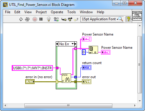 Figure 1. Example of using "Find VISA Resource" VI. If I open up the Keysight (Agilent) Connection Expert software I can see the format of the VISA address and this matches the format string I’m inputting to the Find VISA Resource VI. The string is basically this format for all USB instruments, but the key here is that this instrument’s serial number always starts with “MY” including that plus the search question mark plus wild card should keep this code from finding the wrong instrument. Plus, I don’t expect any other Aglient instruments to be connected to this system. 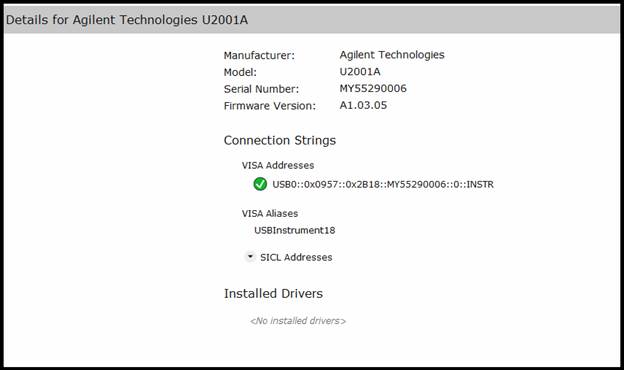 Figure 2. Screenshot from Agilent connection expert - shows VISA address string for USB instrument. I feel this is a good fix for having to provide an alias in NI MAX. However, I have noticed that this will not work with NI hardware like a DAQmx usb instrument. It shows up like this. 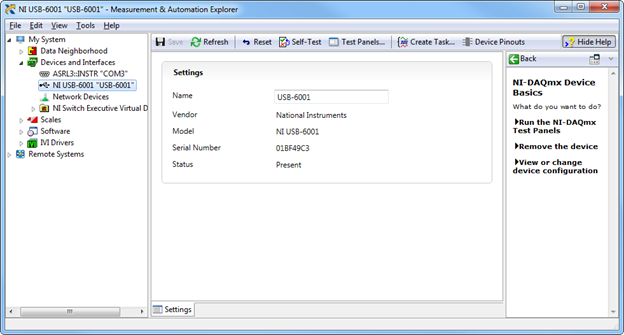 Figure 3. Example of DAQmx in NI-MAX. From what I read here DAQmx does not use at resource string scheme like other instruments. This page and example shows to use this NI-ModInst tool. I have not used it for real, but just looking at it quickly it appears to only find PXI instrument. It is not seeing my USB DAQmx instrument. 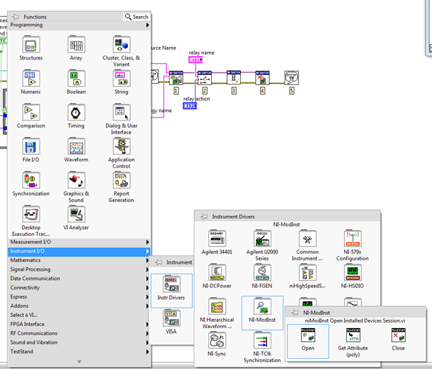 Figure 4. Location of NI-ModInst tool. 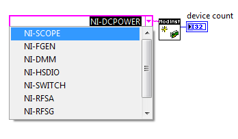 Figure 5. Instrument options that ModInst provides - PXI instruments. Digging a little more a DAQmx device name can be found with the DAQmx System Property Node. See here. Here is how to get to it and you can see it returns the device name alias. 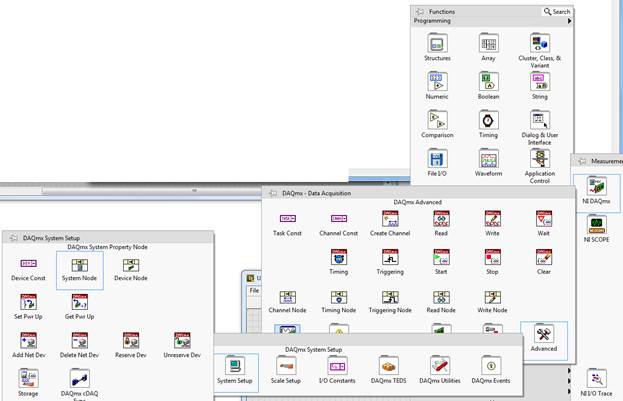 Figure 6. Location of DAQmx System Property Node. 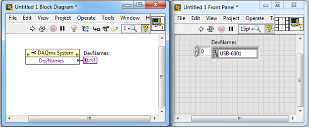 Figure 7. Use the DAQmx property node to get the device name. What you can do with this is make this VI contain a control with the name and send this into TestStand as a variable. All set.
0 Comments
In part 2, I talked about preconditions, post actions and some other ways to add limits to tests. In this part I’ll continue looking at some of the other step types, specifically:
Creating a sub-sequenceIf you have ever read anything National Instruments puts out on good code development practices they always talk about coupling and cohesion. That is, making code modules that are loosely coupled and have high cohesion. Coupling means that code modules are for the most part independent and not too “coupled” together. Cohesion means that the all the code in one module is there to perform the one purpose of that module. One way to build cohesion into a TestStand sequence is to make the separate tests (or whatever logical division you are using) into their own sequences. You can either have a sequence file call other sequence files or you can create a subsequence that is called from a main sequence. The difference between the two is that subsequence is not visible in file directory, it’s just stored in the main sequence. Starting with the TSBasics2.seq sequence file from part 2 and renaming it TSBasics3.seq, I’ll show how to turn the Sine Amplitude and Frequency Test into a subsequence. Figure 1 shows the sequences pane, right click and select insert sequence. 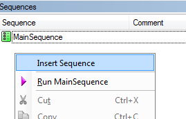 Figure 1. Inserting a sub-sequence in the Sequences pane. Name the new sequence AmplitudeAndFrequencyTest. Cut and paste the steps from the MainSequence into the new AmplitudeAndFrequencyTest sequence. At this point this new sequence is still not called, so we have to drag a sequence call step from the Insertion Palette into the MainSequence and set it to call the new AmplitudeAndFrequencyTest sequence. Rename the sequence call, as shown in Figure 2, right click and select Specify Module. Then, click on the Use Current File check box and select AmplitudeAndFrequencyTest from the drop-down list as shown in Figure 3. 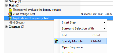 Figure 2. Specify the sequence you want to call with a Sequence Call step type. 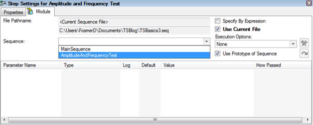 Figure 3. Select the AmplitudeAndFrequencyTest sub-sequence to call. There is one more thing to fix. Since we used local variables in the main sequence to move the amplitude and frequency measurements into the limit steps, we have to put those local variables in the new AmplitudeAndFrequencyTest subsequence. These can just be cut and pasted from the main sequence. Message popup and passing parametersNow that we have a subsequence in order to interact with this subsequence in a way that maintains good cohesion we have to add parameters to the subsequence. First, let’s use the Message Popup step type that will allow the user to set the stimulus frequency. This message popup will set the users input to the local variable called StimulusFrequency. Then we will add a parameter to the AmplitudeAndFrequencyTest subsequence called SetStimulusFrequency which will be passed to the VI for testing and we will see the result on the report. Add the message popup step type (Figure 4) 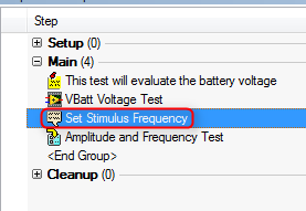 Figure 4. Adding a message popup step type. Create a local variable in the main sequence called StimulusFrequency. On the message popup, rename it to “Set Stimulus Frequency” and go to the Expressions tab of the step properties. Add the Post-Expression, Locals.StimulusFrequency=Val(Step.Result.Response) as shown in Figure 5. This will assign the user response to the local variable and the Val function will convert the string to a number. Go to the Options tab of the Message popup and click the Enable Response Text Box option. This is what allows the user to input a value. 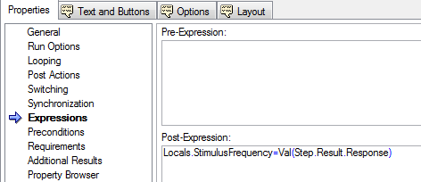 Figure 5. Adding a variable for a response text box type message popup dialog box. The next task is to go into the Amplitude and Frequency Test sub sequence and create a parameter called SetStimulusFrequency shown in Figure 6. This will be how the sub-sequence is passed the stimulus frequency from the upper level main sequence. 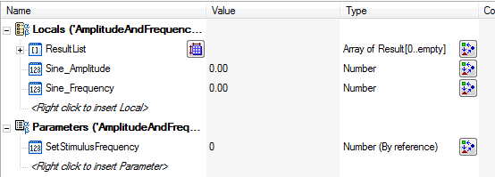 Figure 6. Adding a parameter to allow passing data from the main sequence to the sub-sequence. To add this as a parameter, from the MainSequence we click on the Amplitude and Frequency Test sub-sequence. Select the SetStimulusFrequency parameter and use the Value field to set the value that will be passed to it. Here we are using the local variable StimulusFrequency. See Figure 7. 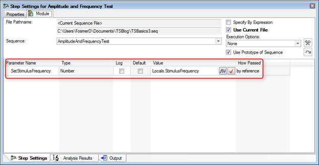 Figure 7. Setting up the local variable that will be used as the parameter to pass into the sub-sequence. Another thing we should do when adding user input is validate that input. The user input is accepting a string and we are converting it into a number, we should make sure that is a valid number. Right now the limit on frequency is 4999 to 5001, let’s open that up to 1000 to 10000. I’ll make two locals holding these values, 1000 and 10000. Then I’ll add a status expression to make sure the entered value is within this range. Figure 8 shows the expression. If the input is not in this range, then the step fails and we’ll add a post action to repeat the step on failure shown in Figure 9. 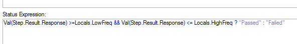 Figure 8. Expression to check if the user input is within the acceptable bounds. 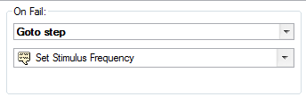 Figure 9. In the event of an invalid input the dialog will popup again to ask the user for input. We also have to go the Run Options tab in Figure 10 and uncheck the Step Failure Causes Sequence Failure option, or any incorrect entry will cause the test to fail. Now, if you enter a number smaller or larger than 1000 to 10000, it will just pop back up to reenter. This isn’t totally fool-proof, for one thing there is no dialog explaining that you entered an invalid value and you could probably enter text into the dialog that would convert to a number in this range and the sequence would pass with some random input. Another problem is the validation values are not tied to the actual limits, so there could be a mismatch. So… room for improvement.  Figure 10. Uncheck the option that step failure causes sequence failure. Failure here indicates incorrect input not test failure. This last step also gave us a chance to write some expressions. Expressions are very powerful, but I’ve found they can be tricky and the help isn’t always easy to find. The expression browser shown in Figure 11 is probably the best bet and a lot of experimenting and learning has to take place. 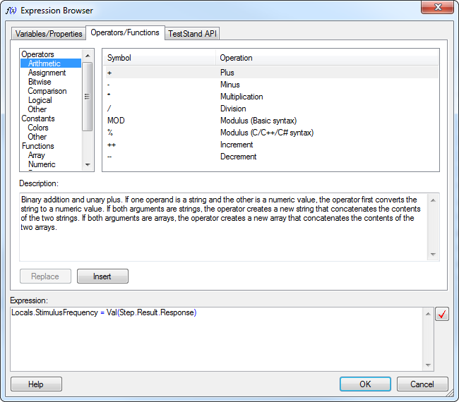 Figure 11. Expressions can be extremely complex, the Expression Browser provides help and context to writing them. Using the Property Loader The last thing I’m going to look at today is the Property Loader. The Property Loader is a step type that will load properties from a file or database. This is super-useful because you can keep things like your test limits in a separate file and change them without having to change the sequence file itself. It’s pretty easy to set this up, I’ll demonstrate with loading properties from Excel. First drag a Property Loader step type into the Setup step group of the main sequence. This is the perfect type of operation to put into the Setup step group of the as it fits well into the logical category of setup. Since we already have all are limits setup in the sequence file and sub-sequence it’s easy to create the limits Excel file. Click on Tools -> Import/Export Properties… On the Source / Destination tab select file and Excel, on the Properties tab select all sequences and click the limits button. Click Export, give it a file name and click done. See Figure 12 and 13. 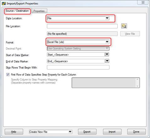 Figure 12. Set the file type to Excel for the Property Export operation. 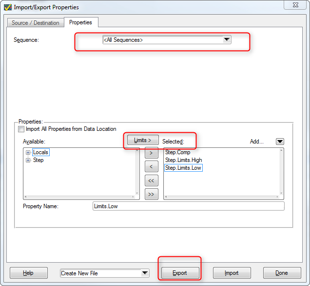 Figure 13. Selecting limits as properties to be exported to an external property loader file. Now let’s take a look at the file that was created in Figure 14. You can see that the limits we previously setup are in there along with empty fields for locals, file globals, and station globals. 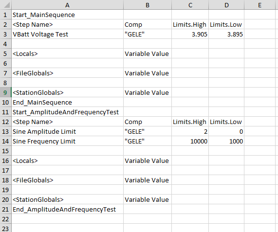 Figure 14. Excel file result of the property loader export function. Going back to the main sequence, click on the Property Loader step we added and click Edit Property Loader… in the step settings. Make the settings shown in Figure 15 for the Properties tab and shown in Figure 16 for the Source tab (navigate to your property file you created as your file path will be different). 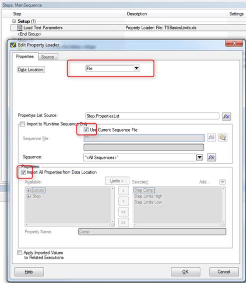 Figure 15. Property loader step type settings. 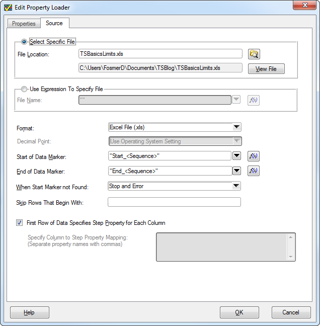 Figure 16. Property loader step settings for data source. Next thing I added, that is optional, is a message popup to the AmplitudeAndFrequencyTest sequence to show the limits that were read from the limits file. Figure 17 shows the expression needed to create this popup message. This is just to illustrate that the limits are being pulled from the file at this point and not what is saved in the sequence file. We don’t have to do anything to the sequence file to get the limits applied to the test results, that’s all handled in the property loader. One thing we may want to do is simply zero out the limits in the sequence file so no one is tricked that the limits are stored there. This may call for a Label comment as well. The bad thing about zeroing the limits is now when you read the sequence file the descriptions would just list limits of zero. So, it’s up to you what you like. 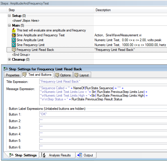 Figure 17. Expression that reads back the frequency limits as loaded with the property loader file. SummaryThat’s all I’m going to go over in this post. I worked through adding a sub-sequence with a parameter, a message popup and wrote some statements to validate the input. I also showed the basics of using the Property Loader to load limits and other values from an external file. Source CodeFind the code for this post here RelatedIn Part 1 on TestStand I programmed the very minimum to get a test system going. In this part, I’ll add some more steps and show a lot of other useful features. This will mostly involve test steps and flow control. Using A PreconditionThe first thing I did was add a new test VI, a battery voltage test. Note again that this isn’t a real measurement, but for this one I added a little randomization so the results are somewhat more of a realistic simulation. Figure 1 shows the battery voltage test VI. 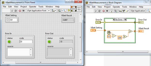 Figure 1. VI to simulate a battery voltage test. I have added this new test to my sequence file before the sinewave test, this time I used the Numeric Limit Test adaptor as this VI has only one output that I want to apply a limit. You can see from the code above that the maximum range the simulated VBatt Result can be is 3.895 to 3.905, so that is what I set the limits to. It’s slightly easier to setup the Numeric Limit Test than it is to setup the Multiple Limit Numeric Test. First I go to the Limits tab of the Step Settings to enter the high and low limit as shown in Figure 2. Next I went to the Module tab and set the VBatt Result Value expression to be Step.Result.Numeric. This is shown in Figure 3. This again is using TestStands built-in results collection. That it, then the Data Source tab is automatically set to Step.Result.Numeric as well. 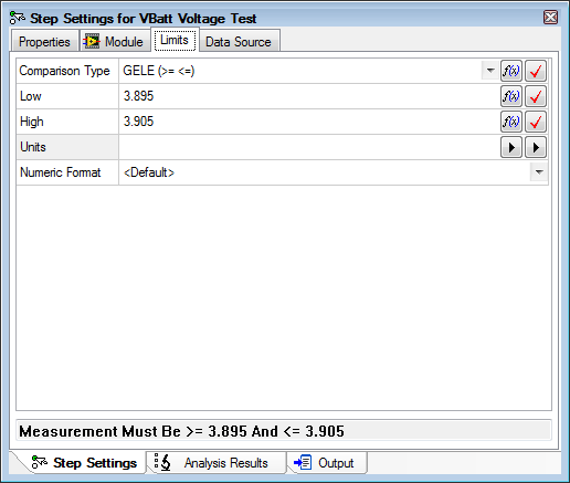 Figure 2. Setting high and low limits for the battery voltage test. 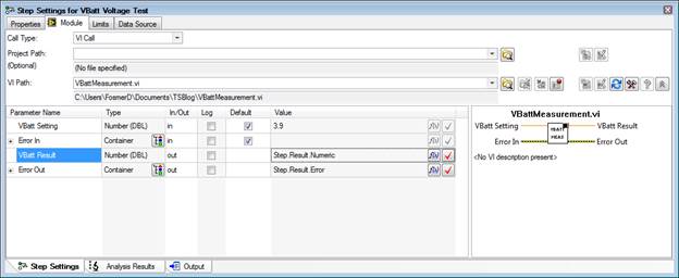 Figure 3. Linking the battery voltage VI result to the TestStand results collection. The next thing I’m going to do is apply a precondition to the sine amplitude and frequency test. A precondition is an expression that is evaluated before a step executes. I’m going to create a precondition that says the Sine Amplitude and Frequency Test will only execute if the VBatt Voltage Test passes. Since this is such a common task there is a very quick way to write this expression. Go the Sine Amplitude and Frequency step and go to the Properties tab of the step settings. Click on Preconditions and click the Precondition Builder icon shown in Figure 4. 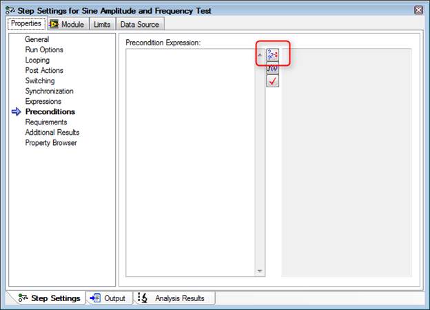 Figure 4. Location of the Precondition Builder icon. In the Precondition Builder dialog box click the VBatt Voltage Test step, then click Insert Step Pass button and that’s it. This is shown in Figure 5. 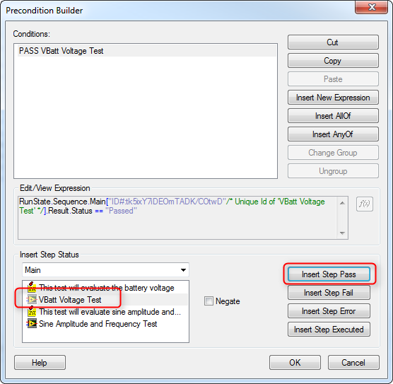 Figure 5. Setting a precondition that the VBatt Voltage Test pass for the Sine Amplitude and Frequency Test to be run. Save the sequence file and in the Execute pull down menu click Single Pass. The sequence will run and you can see from the report that both the VBatt Voltage and Sine Amplitude and Frequency Tests pass. To test the precondition we can force the VBatt Voltage Test to fail. Right click on the VBatt Voltage Test step and click Run Mode -> Force to Fail. You can now see in Figure 6 the settings for that step it is set to Force Fail. Run Single pass again and we can see the Sine Amplitude and Frequency Test is never run and set to a status of skipped. Figure 7. 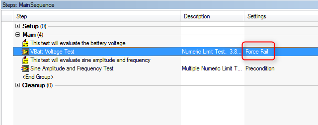 Figure 6. Set the VBatt Voltage Test to Force Fail in order to test the Sine Amplitude and Frequency Test precondition. 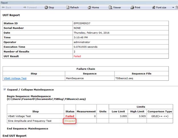 Figure 7. The test reports shows that the Sine Amplitude and Frequency Test was skipped due to failing the precondition. Using a Post Action instead of a PreconditionThere are lots of ways to do things in TestStand. For example, I’ve worked with some engineers who don’t like to use preconditions because they feel it hides test flow inside the test step where you can’t see it. A way you can avoid preconditions that also saves quite a bit of work is to just program the conditional step to go to cleanup on fail. Say there were 4 other tests along with the Sine Amplitude and Frequency test and we don’t want any of them to execute if the VBatt Voltage Test fails, we can just tell the sequence to go to the cleanup step on failure of the VBatt Voltage Test and we can skip all the preconditions. Here under the Post Actions property you can see in Figure 8 we’ve left the behavior for on pass to default as go to the next step, but changed the on fail to go to step cleanup. 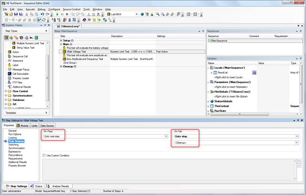 Figure 8. Setting up a post action to go to clean up on step fail. Making limits their own stepAnother method to set test limits is to make them their own test step. This can be nice because if you have multiple limits in one sequence step they are hidden away and not easily view without opening the step. Putting each limit as its own step makes it a little easier to read the sequence. This will also demonstrate the concept of using a variable, which we have not talked about yet. Here is the process to move the Sine Amplitude and Frequency Test limits to their own sequence steps:
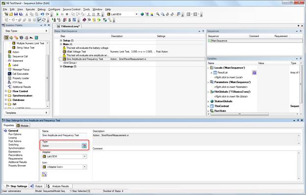 Figure 9. Changing the type for the Sine Amplitude and Frequency test to an Action rather than a numeric limit test. 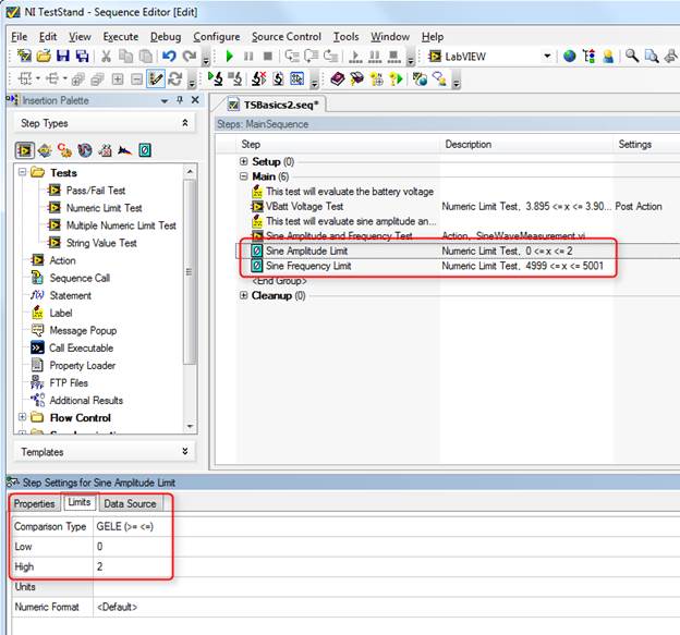 Figure 10. Adding two Numeric Limit Tests for amplitude and frequency with the adapter changed to none. 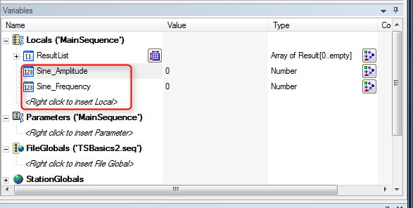 Figure 11. Add local variables as a way to store the amplitude and frequency measurements. 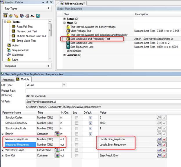 Figure 12. Connecting the output of the Amplitude and Frequency measurement VI to the local variables. 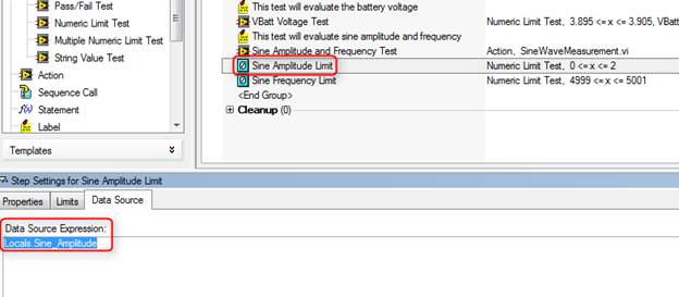 Figure 13. In the limit evaluation steps - set the data source to the local variables. Now if we run the sequence you can see in Figure 14 that it still passes. 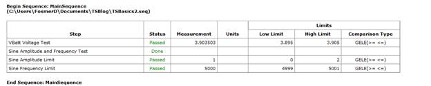 Figure 14. The test report shows the amplitude and frequency evaluation is now in the new sequence steps Improving the format of the test reportOne thing I noticed in the report is all those digits in the VBatt Voltage Test and the Sine Amplitude and Frequency are not in the correct format. If I go to Configure -> Results Processing I can change the way numbers are reported on the report. Figure 15. 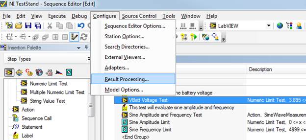 Figure 15. Open the Results Processing dialog box. In the results processing dialog if I click on options then I can edit the number of digits on the report as shown in Figure 16. The default number of digits is 13. 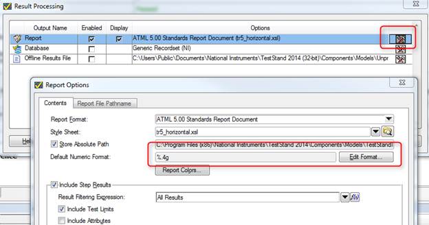 Figure 16. Changing the number of digits shown on the test report. I also noticed that the limits on amplitude and frequency should have some digits. Go into the limit step and add a custom numeric format. I also added a unit of measure, which makes it look a little better, see Figure 17. 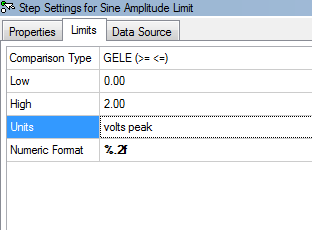 Figure 17. Setting the number of digits that are displayed on a limit. We also need to go update the local variables to keep them from cutting off any digits. Right click on the amplitude and frequency variables and change them to Real with two digits of precision. Figure 18 shows the Numeric Format dialog box. 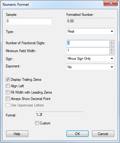 Figure 18. Adjusting the numeric format of a variable. I also went back and added a unit for the VBatt test. Now in Figure 19 our report is looking a little bit better. 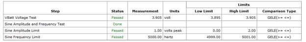 Figure 19. Updated test report after adjustments for number formatting and adding units. SummaryIn this post I showed some different methods to control the flow of the test with preconditions and post actions. I also showed how to use local variables rather than the automatic results built into TestStand to apply limits to tests. Finally, I showed a couple little things to format the test report. Source CodeFind the code for this post here RelatedIntroductionOver the last year or so I’ve been working with NI TestStand quite a bit. While, I’ve worked with LabVIEW for several years, I have not had much exposure to TestStand. I’m hoping to write a blog series on TestStand to aid in my learning. When I started using TestStand my first question was, “how do I use this to make the creation of a test system faster?” I wanted to use LabVIEW and get a test system up and running quickly but I didn’t have any test executive infrastructure in place. That is I just wanted the operator interface, test sequencer, and report generation done so I could focus on tests. Well, that’s what TestStand is supposed to do and I was going to figure out how to make it do it. Unfortunately, I didn’t know much about TestStand and I had to figure out how to do all the basic stuff. NI always has lots of training materials available, but I just wanted to know how to get something super simple going, and I couldn’t quite find the help I wanted. If you start with an empty sequence file it looks like Figure 1. 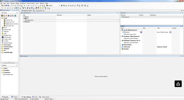 Figure 1. Empty TestStand sequence Navigating the TestStand Sequence EditorOn the left is the Insertion Palette, note in Figure 2 I’ve pointed out the Module Adaptor selection area. I have mine set to LabVIEW as I want to call my labview code on each test step. Other choices are C/C++ dll or .NET. Simply click on these to change the adaptor. There’s lots of other useful stuff in the Insertion Palette I’ll talk about later. 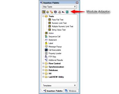 Figure 2. Module Adaptors on the Insertion Palette Another area of interest is the Steps Pane. That’s right in the middle and controls your test steps and test flow. Figure 3 shows the Steps Pane. I think the Steps Pane is technically held in the Sequence File Window. I don’t know, these terms aren’t that important. 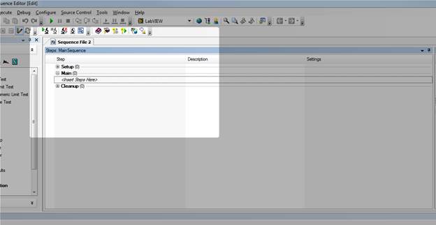 Figure 3. Steps Pane of the Sequence Editor. Off to the right is the Sequence Pane and the Variables Pane. Figure 4 shows the variables pane. 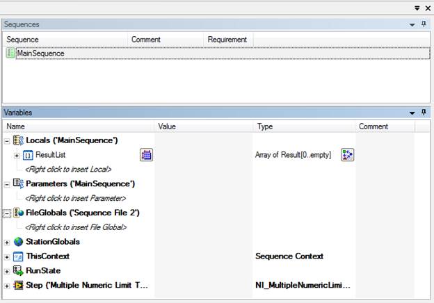 Figure 4. Variables Pane of the Sequence Editor. You’ll see that dealing with all these panes and windows can get to be a pain (I’m so funny). There are a lot of ways to move and dock all these windows. You can even pull some of them out of the sequence editor onto the Windows desktop on another monitor. So play around with it. Using a Test AdaptorNow let’s say we have some LabVIEW code and we want to run it in TestStand. Based on the code, we will pick one of the standard LabVIEW test adaptors. In this case I’ll chose Multiple Numeric Limit Test since my VI has multiple outputs that I want to evaluate with a limit and it’s probably the most useful one. In Figure 5 I dragged the Multiple Numeric Limit Test from the Insertion Palette to the Steps Pane under the Main section. 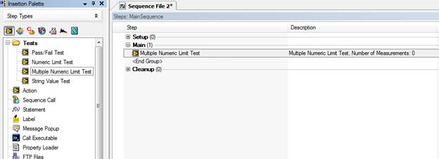 Figure 5. Use of the Multiple Numeric Limit Test adapter. Clicking on the new Multiple Numeric Limit Test, we can see in Figure 6 that the Step Setting pane is now populated with several tabs and settings options. I’m going to click on the Module tab and browse for the VI I want to run. 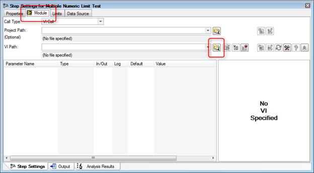 Figure 6. Selecting a module for the Multiple Numeric Limit Test adapter. The VI I am loading is just a simple sinewave generator I wrote up quick in LabVIEW. Its outputs are the sinewave amplitude and frequency. I’m going to pretend that this is my test data. See Figure 7. 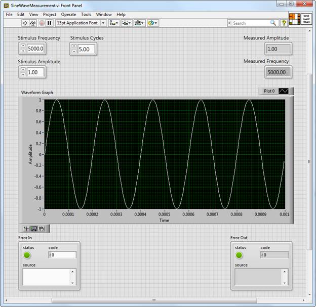 Figure 7. Front panel of sine wave measurement VI that will be used in the sequence. Now that the VI is loaded into the test sequence let’s setup TestStand to run the VI and apply limits to the measurement results. There are multiple ways to do this, the first way I know is to use the built-in results collection of TestStand. Start on the Limits tab shown in Figure 8, and use the plus sign to add two measurements. Change their names to “Amplitude” and “Frequency” or whatever makes sense. 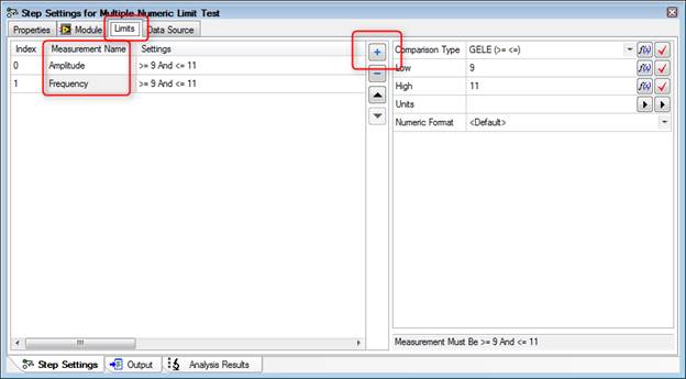 Figure 8. Applying limits to the amplitude and frequency outputs of the test VI. Next go to the Module tab shown in Figure 9 and click on the Expression Browser button in the Measured Amplitude parameter row. 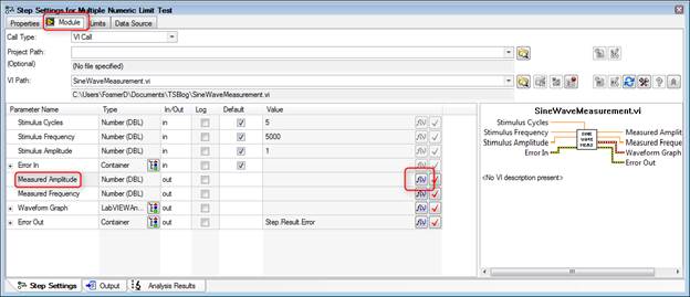 Figure 9. Accessing the Expression Browser for the amplitude output of the test VI. Once you click on the Expression Browser button you’ll see the Expression Browser dialog box shown in Figure 10. What we are trying to do is map the output of our VI to the result collection measurement name we created when we added the amplitude and frequency limits. Browse into Step -> Result -> Measurement -> [“Amplitude”] ([0]) -> Data and then click on Insert and OK. 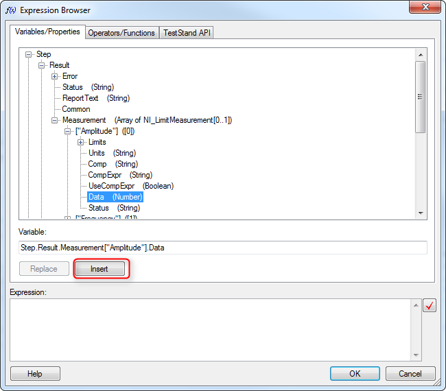 Figure 10. Connect the amplitude output from the test VI to the sequence file to be used in the limit evaluation. Go to the Data Source tab as shown in Figure 11 and click the check box called Specify Data Source for Each Measurement. Under Data Source there are two lines one for the amplitude and one for the frequency measurement. Here we are connecting our data from the TestStand results collection to the limits to be evaluated. Figure 12 shows how to use the expression browser to create the statements shown in Figure 11. 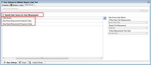 Figure 11. Connect the data source to the test step to be evaluated as limits. 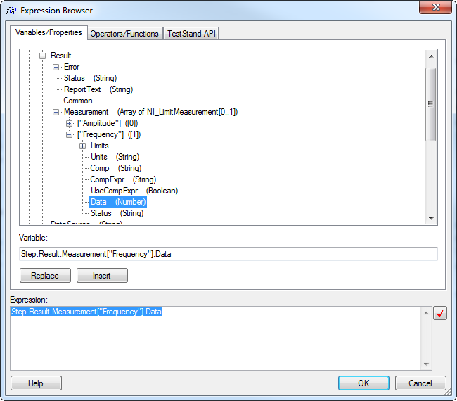 Figure 12. Using the Expression Browser to create the data source statements. Now go back to the Limits tab shown in Figure 13 and set the limit span. In my VI, the default amplitude is 1 and the frequency is 5000. As you can see there are several options for one or two sided limits, inclusive and so on. I chose GELE and selected the units. 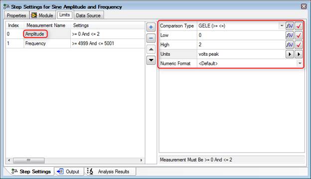 Figure 13. Options to set the limits amplitude limits, comparison type, low, high, units and numeric format. Returning to the Steps Pane, name the step something like “Sine Amplitude and Frequency.” Also, drag a label from the Insertion Palette as a way of documenting this step. The Label step type is shown in Figure 14. 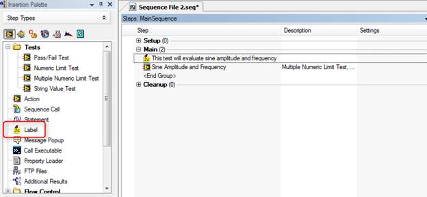 Execute the SequenceWe are actually pretty close to a complete test system at this point. It might not test much but we can now enter a DUT serial number, execute the sequence and get a report. In the Sequence Editor, click Execute-> Test UUTs, the UUT Information dialog box in Figure 15 will appear to enter a serial number for the part. Also, if you have a UBS bar-code scanner attached to the system it will automatically accept the input into this dialog box field. I didn’t know this, but a USB bar-code scanner will read text into most software, it’s just like a keyboard or mouse. You can even scan right into Excel. 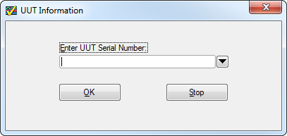 Figure 15. The UUT Information dialog box built into TestStand Type something in there like “1234” and click OK. TestStand will execute will show that the test sequence passed. The little dialog box that pops up that says “Test Sequence Passed” is shown in Figure 16, this dialog is controlled and created by the process model (so is the UUT Information, for that matter). 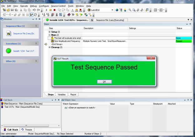 Figure 16. UUT Result dialog box shown after test run pass. Click OK on the UUT Result dialog and click Stop on the UUT Information dialog box. The test report will pop-up and you can see all the information and measurements that are collected. It’s a pretty good report right out of the box. Figure 17 shows an example of the report. 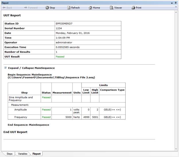 Figure 17. Example of the default sequence report created by TestStand Each time the test is executed the report will be saved in xml format to the directory in which your sequence file is saved. One last step to creating a fully functional test system is adding a user interface. The TestStand sequence editor allows you to run the sequence and your test, but it’s not setup to do real testing by a test operator. TestStand comes with premade test system user interfaces to solve just this problem. Before we look at the user interface we have to create a user with limited permissions to be our operator. In the sequence editor click View -> User Manager. Under the Users section right click and add a user called TestOperator. Right click this new user and select Properties, and click Operator. See Figure 18. 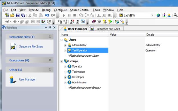 Figure 18. Creating a Test operator user profile in the TestStand user manager. Save the new user setting and close the User Manager. Note that the User Manager changes are a station setting and live with the installation of TestStand on the computer you are using, and are not saved into the sequence file. Go to this path C:\Users\Public\Documents\National Instruments\TestStand 2014 (32-bit)\UserInterfaces and you will find two folders, Simple and Full Featured. In these folders you’ll find the premade user interfaces in a variety of languages. If we go in Full Featured and LabVIEW you’ll find a file called “TestStand 2014 (32-bit) LabVIEW UI – Operator” this is the LabVIEW implementation of the user interface. From this interface you can then load your test sequence file and run it in a production environment. As shown in Figure 19, open the file and login as the new user TestOperator, then open the sequence file that we built and you are ready to test by clicking the Test UUTs button shown in Figure 20. 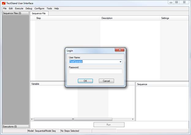 Figure 19. The TestOperator login in now available. 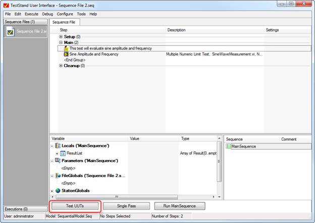 Figure 20. Begin testing by pressing the Test UUTs button. SummaryTestStand is a great tool to building a simple test system quickly as it handles a lot of the infrastructure for you like, user interface and reporting. This was the super basic stuff to load a LabVIEW VI and run it in the TestStand sequencer. TestStand can sort-of be as sophisticated and complex as you want it to be as you become more of a power user. I’m still a beginner, but I will keep writing as I learn and hopefully it will be a benefit to some others and I’ll remember how to do stuff the next time. RelatedRecently I’ve been working with the Agilent U2001A power sensor. The U2001A is an averaging power sensor which simply means when the instrument is queried, that result is an average of multiple samples. If you want to easily measure peak power, you have to purchase the U2020 series power sensor, which costs more. However, the U2000A averaging sensor can be configured to create what is called a trace graph display, which effectively queries all of the individual points that go into the averaging the sensor is performing. Finally, software can be used to find the peak power measurement or simply display the measurement like a digitized waveform. To determine how to create the trace graph display I used the U2001A programming guide and the U2000 Series Labview driver from NI. The Agilent programming guide provides the example code, shown in Figure 1, to create a trace graph display. 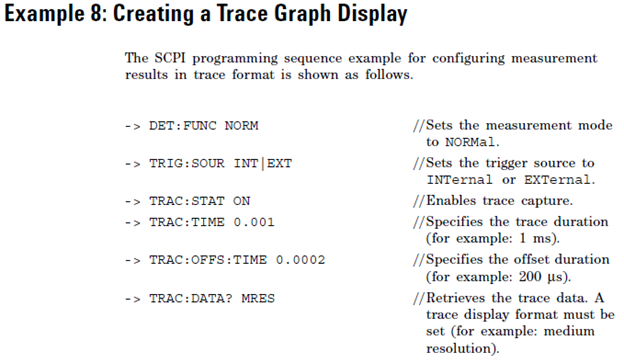 Figure 1. Example code for creating a trace graph display from the Agilent programming guide. This code is basically correct, but I feel like they left out a couple things. First of all I found that the trigger requires a little more explanation. The best way I found to do it was to trigger on a power level, their example doesn’t have this code. If you do not specify a trigger level it will just trigger immediate, but this doesn’t give as much control in some situations. Another thing I struggled with was how to decode the data returned by the instrument. The data is returned from the instrument in something called the IEEE 488.2 arbitrary block program data format. It took me a little while to find it, but the LabVIEW driver includes a VI to decode this data. I’m just pointing this out because the example from the programming guide doesn’t go into these details. Figures 2 and 3 show the LabVIEW code. The actual code is also available. 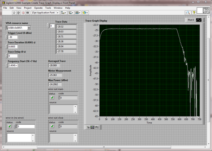 Figure 2. Front Panel of Example Create Trace Graph Display VI. A couple of things to note in Figure 2, the trigger level was set to -30 dBm. You can see from the graph that the acquisition begins at -30 on the rising edge of a pulse, there is a flat portion, and falls back into the noise. Also note the VI outputs: “Averaged Trace” is the average of everything on the graph, “Meter Measurement” is the average returned by the meter (I’m not totally sure why that doesn’t match the average computed in the software – I think the points acquired and the measurement points must not match) and “Max Power (dBm)” is the peak value found in the graph array data. 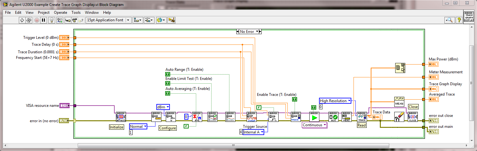 Figure 3. Block Diagram of Example Create Trace Graph Display VI. Figure 3 shows the block diagram of the example LabVIEW code. This code has quite a bit more configuration than the example code from the programming guide in Figure 1. Figure 1 shows the critical command and many of the extra commands I have in the LabVIEW code can be stripped out as they are just resetting the default values – I just felt this was more complete. As I mentioned earlier, one nice thing in this code is the U2000 driver implements the code to read the trace data. This capability is in the VIs “Read Trace.vi” and “Parse Data.vi” which are shown in Figures 4 and 5. You can also see that the driver has a comment with some details about the IEEE 488.2 data format. 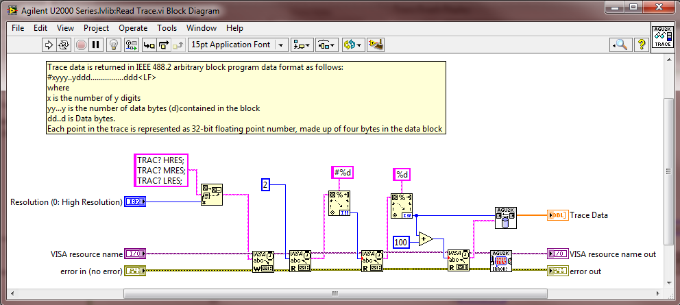 Figure 4. Read Trace.vi. 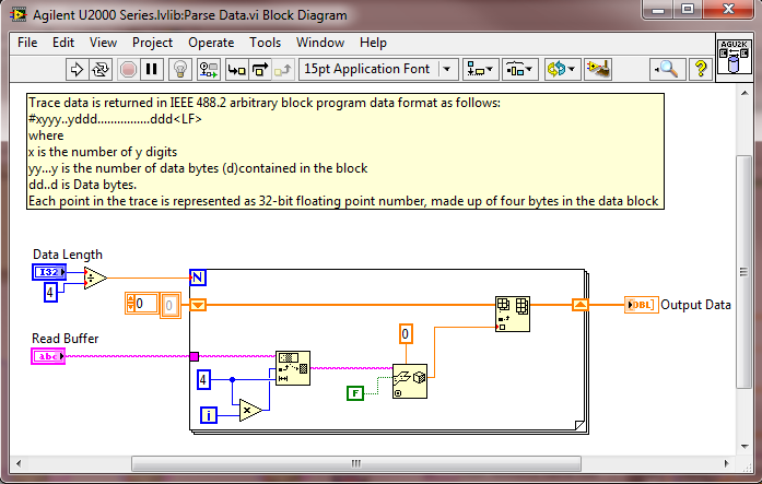 Figure 5. Parse Data.vi. One strange thing I found with this code is it seemed to work great if I kept the sub-VI “Wait for Acquisition Complete.vi” open, but if it was closed it seemed like code would hang-up a lot. Not sure what that is all about.
I posted this example code and you can download on this page, it is LabVIEW 2012. Note that I’m not providing the U2000 driver, get that from NI at the link above. Summary This post shows how to implement an Agilent U2001A power sensor trace graph display in LabVIEW. I feel this code provides a slightly more complete solution than the example code provided in the Agilent Programming Guide. Another useful feature of this code is it makes it possible to find the peak power of a measurement using the average power model power sensor. A while back, actually quite a while back, I decided to start adding some test engineering related projects to this site. The first one I took on was developing a test executive from scratch in Labview. I realize that NI has the TestStand product that is an off-the-shelf test executive. I have not used TestStand in years simply because my company does not currently use it. I’m sure what I’ve developed is no match for TestStand, but there is room for developing your own test executive. Some reasons may be you don’t want to pay for TestStand (although it will cost you time and effort to develop your own). Perhaps TestStand is overkill or maybe it will not meet your needs. Basically, developing a simple test executive was a good test related project that would require fairly extensive user interface development. I’ve given my test executive a name, the DOT-TE or Dana On Test Test Executive. That seems a little more cute and clever than I like to be, but it gives me something to name the VIs. I’ve spent quite a while working on this as I have been working on it in my spare time. Like most engineers, I didn’t think it would take as long as it has. This project is still pretty far from being a stable test executive that could be used in a manufacturing environment. In fact I think it’s at about version 0.1. If you look at the specifications and code there are some features that I have not yet implemented, I could keep working on it before making this post but I just feel like it’s time to ship (so to speak). Prototype The way I decided to tackle this problem was to first create a prototype of the user interface with stubs of the main functions I wanted it to have. I saved the prototype that was created; it’s posted in Projects and Code page in the DOT-TE.zip file as “DOT-TE_Main_UI - Prototype.vi”. The point of the prototype was to get an idea of the look and feel of the user interface and help think of all the functions a test executive would need. The main user interface is based on the Producer Consumer design pattern that comes with Labview. Each button click or menu click puts a message into a queue (producer) and sends the message to execute some related code (consumer). Project Planning After I had the prototype the way I wanted it, I tried to write some specifications. I suppose writing specifications wasn’t all the necessary for a project the only involved one person, but I wanted to make this somewhat a true-to-life project. Here are the original specifications I wrote after I had the prototype. Looking at this, I’ve implemented less than half of this: Specifications log in with different privilege test modes sequence file reports print a report database access db limits db store results db sequence file looping subset testing display status and messages display tests p/f input test information PN SN MN Comment load test button run test button edit sequence edit limits directory storage control setup controls like printing display system messages App Database will hold: Test sequence Limits System Database will hold: Test results/reports Put error messages to the System Messages Obviously, the specifications were nothing elaborate. I just wanted to try to make myself think of all the features it should have. In addition to the specifications, I wrote a program flow to try to map out how the test executive would be used and how it should behave. This expands on the specifications and was a way for me to think and write some notes. I have not edited this from what I originally wrote. Test Starts Internal: - Initialize the menu system - Initialize System Messages - Initialize Test Status, Detailed Results and Test Reports to be blank. - Check for the application database External: - gray out Load Parts, Run Test, Abort Test - System Messages - “System Initialize…” - “System Idle.” Load Test External: - select a test from file dialog - populate the tabs - Test Status Tab - list tests - Detailed Results - list tests - list measurements - System Messages “Test Application X Loading…” “Test Application X Loaded Successfully” - enable Load Parts button - System Messages “System Idle” Internal: Load Test button has been pressed. Go to case “BUTTON – Load Test” Go to the default or current test application directory and display the directories available to load. Display the system message “Test Application X Loading…” Check for a valid test application database Check for a valid sequence file and limits file from the application database Read the limits file from the database and hold it in memory somehow. Read the sequence file from the database and hold in memory somehow. Make visible Test Status, Detailed Results and Test Reports listbox, table, whatever with the tests listed. Test Status - lists the tests - add a test loaded Boolean - add pass fail text and Boolean Detailed Results - list the tests - list all the results by reading from the limits file Load Parts External: - put cursor on the “site” field of Test Information - gray out “Complete” button - once “Complete” is pressed enable “Run Test” button - System Messages “Loading Parts…” “System Idle” Internal: - Put the Test Information into a global - When all required Test Information is entered, enable the Complete button - Enable Run Test button and turn on the Test Loaded Boolean when the Complete button is pressed. Run Test External: - update Test Status after each test with p/f - update Detailed Results after each test with measured values and p/f - update Test Reports tab with report when done - generate overall result on front - System Messages “Test Running…” “Running Test X” “Testing Complete” “Report upload to database: Success/Failure” “System Idle” - while running gray the Exit button Internal: - call each test vi according to the sequence file and execute - determine the result of each test - determine overall result - generate test report - check if printing Unload Test External: - clear Test Status tab - clear Detailed Results tab - System Messages “Unloading Test…” “System Idle” - gray - Load Parts - Run Test - Abort Test Internal: Abort External: - stop testing when current test ends - System Messages “Aborting Testing…” “System Idle” Internal: - read from sequence to determine next test Menus - disable menus while test is running. Other Functions (Options) Print Setup (default off) External: - print on completion - print on fail - print all results summary only - print failing results only Internal: Looping (default off) External: - stop on fail - number of times to loop - System Messages “Looping Enabled” Loop stats while looping Test Subset External: - display all tests for loaded test or display no test loaded - radio button for test to run - select all button Application Directory External: - browse to where you want to load test apps from Tools Test Sequence External: - set the names of the test to run (add, remove test) - set test execution dependencies - select the limits file to use with the test application - select the test application name Limits File Fields: App Number App Name Test name Test ID Limits Part Model Serial Units Database – DOT-TE (maybe just make this a folder where the test reports go in the first version) Holds: Test Reports Database – DOT-Test_App Holds: Table 1 – test sequence Table 2 – limits file Looking back, I didn’t do a lot of this, but I feel like it was worthwhile as part of the process. Operation The project was implemented in Labview 8.5 (I know, I’m several versions behind, but that’s what I have access to at the moment). If you go to the Project and Code page of the website and download the code, everything is included in the DOT-TE.zip file. Within the DOT-TE.zip file the project is controlled by the Labview project file DOT-TE.lvproj. The folder “DOT-TE” can go anywhere, I’ve been putting it right under C:\. The test executive code is in the folder DOT-TE Application. The test application is in the Apps folder. The test application is like the actual test code that would be written to test a DUT. The test application is run on the DOT test executive. The example test application I wrote called DOT-Test_App_00001 includes five test VIs that would test some commonly grouped functionality of the DUT. The five tests output constant values in place of real measurements. There is also some code in the five tests to hook into the test executive and make the measurements accessible to it. Opening DOT-TE_Main_UI.vi it executes automatically to start the UI. The idea of the interface is to follow the buttons on the left hand side, working your way down starting with “Load Test.” Figure 1 shows the UI with all buttons other than “Load Test” and “Exit” disabled. This is the default state. 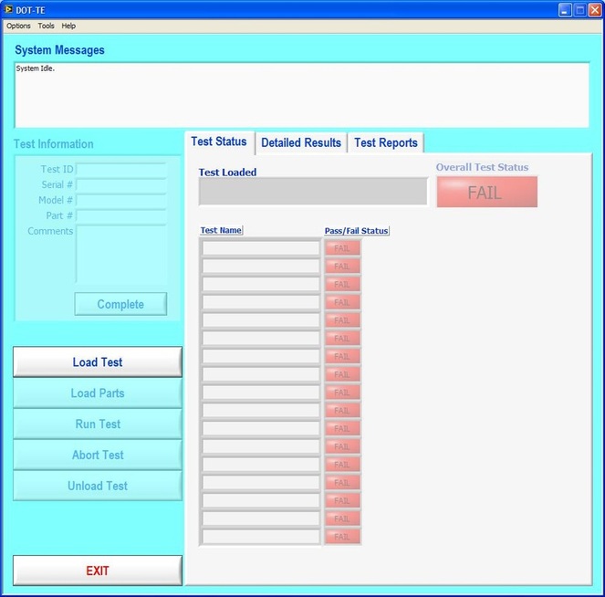 Figure 1. Default view DOT-TE user interface. At the Load Test file dialog select the test application file “Test_App_00001.txt” in Apps\DOT-Test_App_00001, this will load the test application. Figure 2 shows the “Test_App_00001.txt” file dialog. 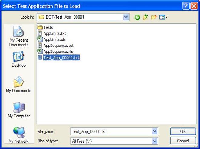 Figure 2. Selection of the application file when “Load Test” is pressed. Pressing “Load Parts” will make the Test ID field of the Test Information active. The test information is how you would identify an instance of the DUT you are testing. The test ID will accept any free text as will the serial number fields. The idea of the Test ID is you would have some system of how to identify a particular test run and enter this there. The serial number would be the serial number of the specific DUT you are testing. Entering the Model # and Part # fields will popup dialog boxes allowing the user to select from the model and part numbers that are listed in the limits file. The purpose of the model and part numbers are just more information to identify your DUT. This is useful, for example, because different model numbers could indicate slightly different DUT configurations. So, two model numbers may have all the same measurements, but different limits need to be applied to those same measurements. What’s nice is there can be a small change to the DUT and the test application and test executive are able to handle it without creating an entirely new test application. Digressing from the UI for a minute, Figure 3 shows the limits file I have mentioned a few times above. 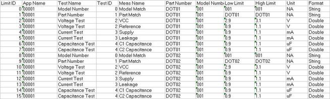 Figure 3. AppLimits.xls limits file The limits file is edited in Excel and saved as a tab delimited text file for the test executive to access. The limits file in Figure 3 has several fields, and five fictional tests. You can see that each line of the limits file is uniquely identified with the “Limit ID” column. This limits file has two instances of the same tests, one for part number DOT01 and another for part number DOT02. I’m not really using the model number as it’s only there to make the possible DUT configurations more flexible. Each test and measurement has a unique name. All the limits are the same for my two part numbers, with the exception of the Model Number test. The app name 00001 comes from the test application name Test_App_00001. The intention is all test application names would take the form Test_App_XXXXX. I guess it’s not that descriptive, maybe that should change. Getting back to the test executive UI and entering the test information. When you tab to the Model # and Part # fields you will see the two dialog boxes in Figure 4 respectively. 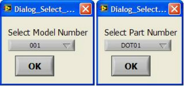 Figure 4. Select Model Number and Select Part Number dialog boxes. Again, the pull down in each of these dialog boxes is populated from the limits file model number and part number columns. Finally, pressing the “Complete” button in the test information section will fill in the information in the “Test Status” and “Detailed Results” tabs of the interface and enable the “Run Test” button. See Figure 5. 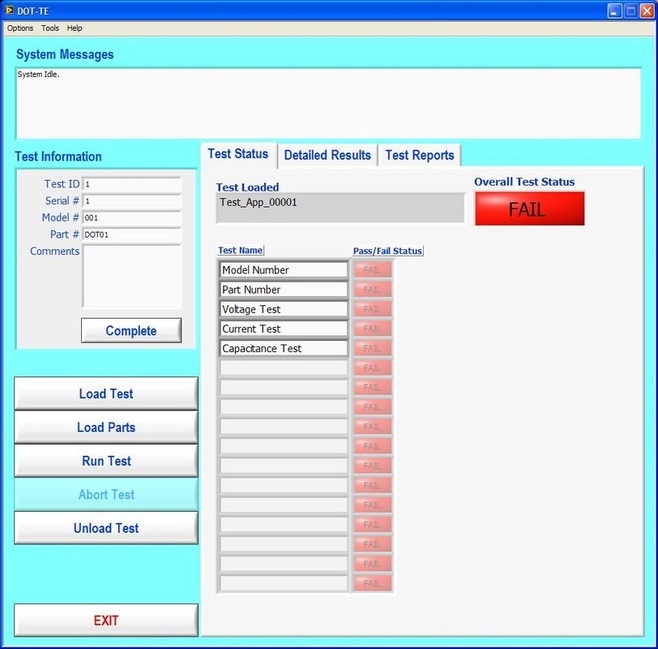 Figure 5. DOT-TE UI with parts loaded and Run Test button enabled. Actually running the test is somewhat anti-climatic because the results are just hard coded for this example test application. Figure 6 shows the directory that holds the test VIs executed when the test is run through the test executive. Again, there a no real measurements happening, but the idea is these VIs would be where you perform the actual measurements on the DUT. You can see in Figure 6 the naming convention I have chosen for the tests. TEST-(test name)-(app number).vi. 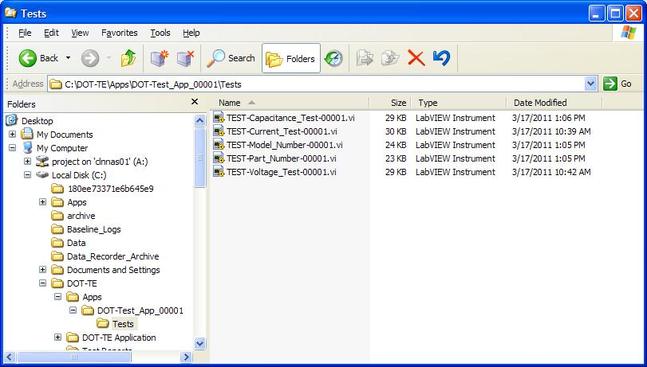 Figure 6. Test application test directory. As a result of running the all the tests, Figure 7 shows the “Test Status” tab with all of the individual tests passing and the overall test status of pass. Figure 8 shows the result of the passing test from the “Detailed Results” tab. The most important information here is the actual measurement data. In the event of a failure, this tab would show you if the test failed high or low relative to the limits or if no meaningful data was gathered (like a test returned NaN). 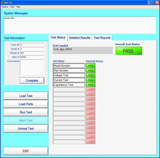 Figure 7. Result of passing test in the Test Status tab view. 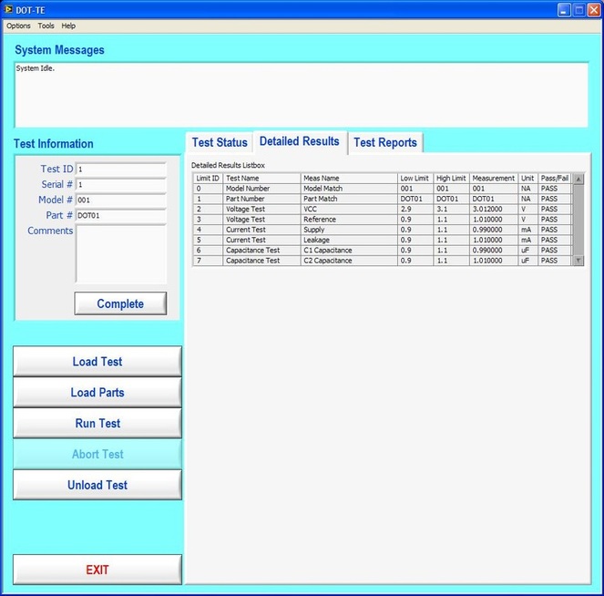 Figure 8. Result of passing test in the Detailed Results tab. At the end of each complete test run an html test report is generated. The test report basically shows the same information that is in the detailed results tab. The history of all the test reports generated since the test executive was opened is in the “Test Reports” tab. Figure 9 shows this. 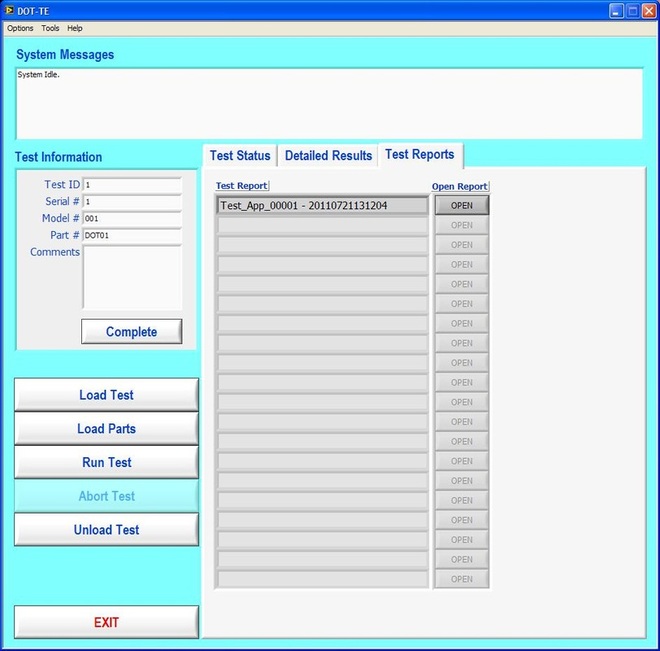 Figure 9. Test Report tab view following passing test. A good enhancement here would be to include the pass/fail status in the test report name. I forgot that. Also, it’s a bit cryptic, but each test report name includes the date and time stamp. At this point, the “Unload Test” button can be pressed and a new test app can be loaded. Or, the “Load Parts” button could be pressed and a new DUT could be loaded and tested. The “EXIT” button unloads the test (if the user forgets to press unload test) and stops the test executive VI running. There are three pull-down menus at the top of the interface: Options, Tools and Help. Options includes sub-menus: Print Setup, Looping, Test Subset and App Directory. Print Setup optionally prints the test report automatically upon test completion. The default is off. Looping is not implemented. Test Subset selects a subset of the tests to run. So, if you have a lot of tests that are very long you can choose to skip some of them. This relies on having an AppSequence file in the test application. Figure 10 shows what is in the AppSequence file. 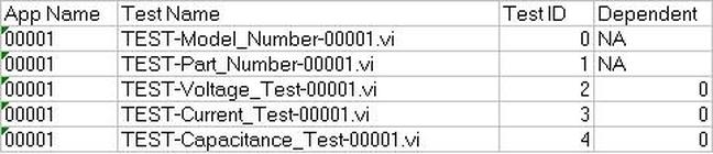 Figure 10 AppSequence file. The AppSequence file also allows dictating test dependency. For example, in Figure 10 if the user tries to run only the test TEST-Voltage_Test-00001.vi without running TEST-Model_Number-00001.vi (where 0 listed in the Dependent column is the Test ID of TEST-Model_Number-00001.vi) an error will be generated from the test executive. The App Directory changes the default location the test executive looks when loading a test application. All options in the Tools and Help menus are not implemented. Implementation I won’t try to go over every detail of the code, if you are familiar with Labview I think it’s pretty simple. Figure 11 shows the project explorer file DOT-TE.lvproj. The project is implemented in one main VI (DOT-TE_Main_UI.vi) with four directories contained all the sub-VIs (Dialog, Globals, Main Functions, Utilities). 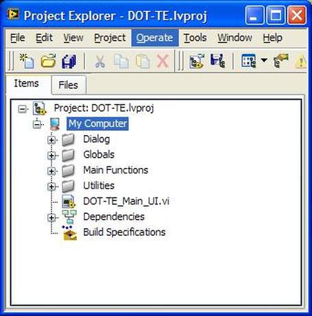 Figure 11. DOT-TE Project Explorer. Figure 12 shows the block diagram of DOT-TE_Main_UI.vi. It may be a little hard to see here, but this is just to see the general producer consumer style. The upper portion contains the event structure that sends a message to the consumer with every button or menu click. The messages are sent with a queue. 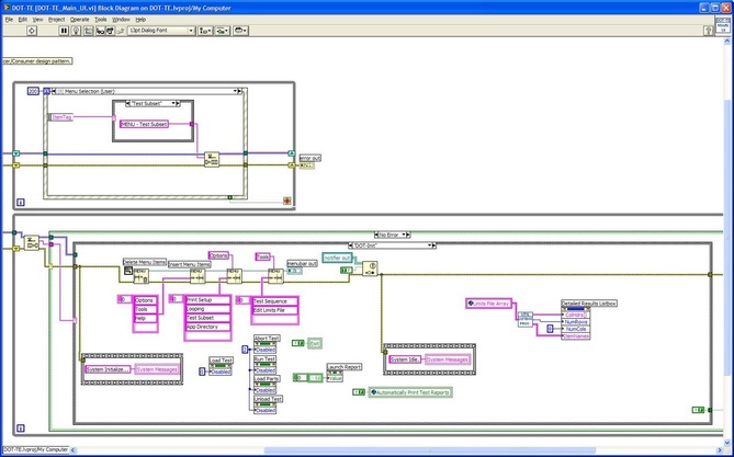 Figure 12. DOT-TE_Main_UI.vi block diagram.
Future Work There is a lot that should happen to this code before it could be really useable. Right now it mostly just demonstrates the concept. There are several places that could be improved. There is no error handling to speak of. The System Messages on the front panel were not implemented. The system messages should be telling the user what’s going on, like when the test is running or the system is waiting on something. Some of the menu features are not implemented. There is very little documentation of the code. Summary A test executive is an important piece of software for a test organization to have in support of manufacturing. While off the shelf test executives exist, there may be cases where a custom design would be worthwhile. The DOT-TE test executive presented here is really about half way done, but it illustrates some important features for a test executive to have as well as some user interface coding concepts in Labview. I have previously written about how to do some basic things with the PXI instruments I have been working with lately. While I covered using the DAQ to generate and acquire analog signals, I would like to expand on what I wrote there. The NI PXIe 6259 M-series DAQ has three kinds of pins, or physical channels, as NI calls them. There are analog I/O, digital I/O and counter pins. The pins are setup like this. 32 analog inputs (ai0…ai31) 4 analog outputs (ao0…ao3) 64 digital pins (Port 0/line 0 to 31, Port 1/line 0 to 7, Port 2/line 0 to 7) where all of these pins are on Dev1. Dev1 is the DAQ, so if you added another DAQ to the PXI chassis it would be Dev2. Port 1 and 2 are arranged like this 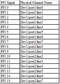 2 counters arranged like this 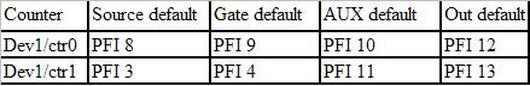 There is also PFI 14 which is FREQ OUT, used as a simple output only frequency generator. PFI stands for “Programmable Function Interface,” which is just a designator they gave it to mean it does something. There is some overlap between the digital pins and the counters. For example, PFI 4 is a dedicated digital pin used for ctr1 gate on counter 1. Digital I/O Example code written to demonstrate digital I/O of the DAQ is shown in Figure 1. The code uses the DAQmx driver to configure a digital input, output and clock signal. The output generates a sequence of digital values and reads them back in on the input when looped back through the matrix PXI card. Counter 0 is configured to be a clock signal where the frequency, duty cycle, initial delay and idle state of the clock are configurable. The digital input is setup to trigger off the clock signal and start acquiring data. The digital output is also setup to trigger off the clock and start generating the programmed data pattern. Notice that the digital output is set to update on the rising edge and the input on the falling edge. This will allow the output level to stabilize before it is read by the input. The clock, digital in and out are all configured to operate with a finite number of samples, 16 used here. It’s a little confusing, but in this case number of samples means clock pulses. Each of the clock, digital input and output are configured with their own task. The input and output tasks are started immediately after the channel is configured, in effect arming the channel as it does not really start until the trigger clock signal is received. Finally, the clock from the counter task is started. This starts the clock sequence and the code waits until the clock is finished allowing all of the digital data to be output and acquired. If I somewhat understand the NI terminology, a channel is created and controlled with a task. For example, you create a digital output channel and then any other code after that related to the channel has to be wired up to the use the same task where the task was created. You can also give the tasks meaningful names to help organize the code. It was a little confusing at first but become pretty intuitive quickly. I guess it’s like the instrument VISA session handles that some older NI drivers used, but you can use multiple tasks within the same instrument.  Figure 1. Digital pattern example block diagram Figure 2 shows the front panel of the code. 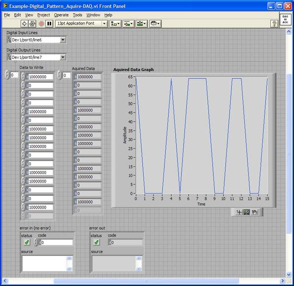 Figure 2. Digital pattern example front panel. In Figure 2 notice that the output and input are configured with only one line, where line 6 is the input and line 7 is the output. These are just arbitrary choices. What is significant is looking at the “Data to Write” array control, in order to set a value of 1 on the output line 7, I need to put a 1 in the 7th bit position (LSB on the right). “Data to Write” is formatted in binary to show this but really the driver accepts a U32 that covers the whole port. The same is true for a 0 value, Labview formats 00000000 as just 0 so it looks a little different than the 1. Also notice, the input line is line 6 so now the bit has moved a position in the “Acquired Data” indicator. You can also see on the graph that the Y axis is in decimal so a high value shows up as a 64. This would probably be a good place to create a new driver where if you are programming a single line only, you don’t have to keep track of the bit position. It’s pretty interesting because there are a lot of possibilities of how you can use this. With some pre-processing you could send a bit stream into a single line (basically, what is happening here) or you can program the whole port at once by just creating a channel as Dev1/port0 rather than Dev1/port0/line7. As also shown, you can split up the port so some of it is configured as input and some as output. Counter The digital I/O example made use of the counter as a clock to synchronize and trigger. The counter can also perform the operations typically associated with a counter, like measuring frequency, period and counting edges. Figure 3 shows the block diagram of an example using the counter to measure frequency. 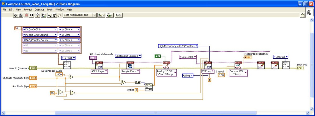 Figure 3 Block diagram measure frequency using DAQ counter The code is very simple. An analog output is connected to a counter input through the matrix. The analog output is configured to generate a sine wave and the counter is configured to measure the frequency. Notice that the programmed sine wave frequency is used to create a max and min value, plus/minus 10, of the measured frequency. This is wired into the counter configuration for accuracy. Figure 4 shows the front panel of the same code. 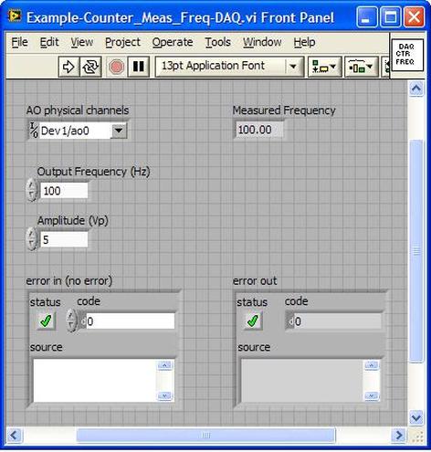 Figure 4. Measure frequency with DAQ counter front panel.
You can see in Figure 4 that the analog output frequency was programmed to 100 Hz and 100 Hz was measured with the counter. Summary This article showed some examples of using the NI PXIe 6259 M-Series DAQ. In addition to analog inputs and outputs the DAQ includes multiple digital I/O lines that could be used in a number of flexible ways. The counter is an additional useful instrument included with the DAQ. The DAQ is marketed as the all-purpose instrument and that’s what makes it interesting to work with. A DAQ can replace a number of more specialized PXI instruments like DMMs and function generators or it could be used to implement very specific high level cards like boundary scan controllers. Recently I’ve been developing a PXIe 1065 chassis based test system using Labview. The chassis includes an 8150 controller, a matrix card, a DMM, a DAQ and some power supplies. It’s a fairly simple set of instruments, but capable of many types of measurements. National Instruments supplies drivers to operate these cards but they require some effort to learn how to put them all together and create working test applications. I’d like to show some examples of how to make some basic measurements and some methods I feel are useful to improve on the supplied drivers. Note that this isn’t the real code I’m writing for my employer since I don’t want to give away any secrets or anything, but it is real working code. Initialization Before any of the instruments can be used to make measurements they all have to have instrument handles established. A good way to do this is by having a test application run an initialize routine that will create instrument handles for all of the instruments and hold them in a global variable. Figure 1 shows the block diagram to initialize the instrument handles for the Matrix, DMM and Power Supply and stores them in a global to be utilized by the application code later. The DAQ is not included, as it doesn’t require a handle to be initialized. The DAQ driver is a little different than the others; I’ll address this later. Figure 2 shows the global variable used to store these handles.  Figure 1. Initialize instrument handles for PXI instruments. 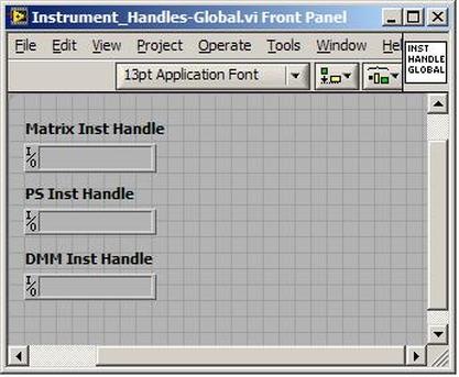 Figure 2. Global variable holding instrument handles (shown un-initalized) Matrix The matrix card is used for switching the instruments to the DUT. I’ve been working with a PXI-2532 16 by 32 crosspoint matrix. Additional hardware has been added as an ITA to make hard connections from the matrix inputs to the other instruments in the chassis as well as the DUT. That is, before you can use the matrix you have to wire the other instruments to the matrix inputs and wire the outputs to your test fixture and ultimately, DUT. Here is where the instruments are connected to the inputs of my system (omitting a couple I’m not discussing) 0. NA 1. NA 2. DMM V+ 3. DMM – 4. DAQ Counter Source 5. NA 6. NA 7. DAQ Analog Out Ch 2 8. DAQ Analog Out Ch 1 9. DAQ Analog Out Ch 0 10. Power Supply Out 2 +20V 11. Power Supply Out 1 +6V 12. Power Supply and DAQ Ground 13. Power Supply Out 3 -20V 14. DAQ Analog In Ch 0 15. DAQ Analog In Ch 8 The two essential Matrix drivers supplied by NI are Connect and Disconnect VIs, as shown in Figure 3. 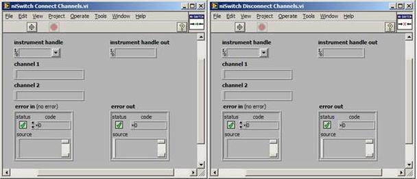 Figure 3. Connect and Disconnect driver front panels. Both VIs simply take the channel 1 input as the matrix input and the channel 2 input as the matrix output you want to connect or disconnect. For the 2532 matrix the input channels are R0…R15 and the output channels are C0…C31. Figure 4 shows and example of connecting the DMM at inputs 2 and 3 to outputs 1 and 2. Let’s say there is a 1k resistor at outputs 1 and 2. 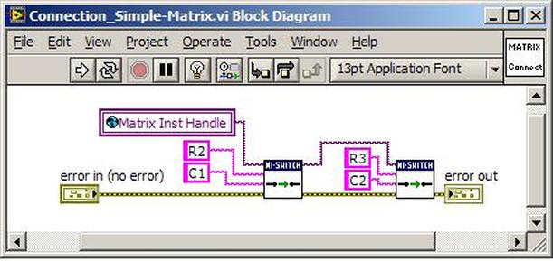 Figure 4. A simple matrix connection The code in Figure 4 will work but it’s not very flexible and it is pretty cryptic as to what is being connected. Some comments could be added to the code to say that the DMM is connected to a 1k resistor. But, a better way would be to create a new driver and give all the inputs and outputs meaningful names using some enumerated types. With a little more work a much more flexible Matrix control can be developed. Then new driver is called, Settings_Advanced-Matrix.vi. Unlike the simple code in Figure 4, it contains three modes: Set List, Clear List and Clear All. It also provides the ability to set multiple input to output pairs at once by accepting an array as input. The input and output designations have been given unique names as controlled by some strict type def controls. The advantage of the strict type defs is that the matrix input and output designations can be updated in one place and all instances of the control elsewhere will update as well. Finally, the code allows for relay debounce by calling the NI driver, “niSwitch Wait For Debounce.vi.” Figure 5, 6 and 7 show the block diagram of Settings_Advanced-Matrix.vi in the three modes. 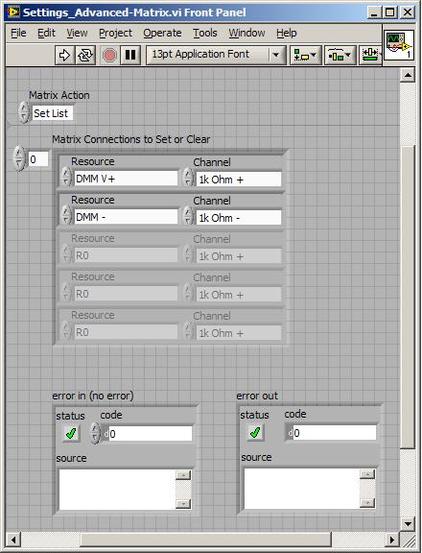 Figure 5. Front panel of Settings_Advanced-Matrix.vi 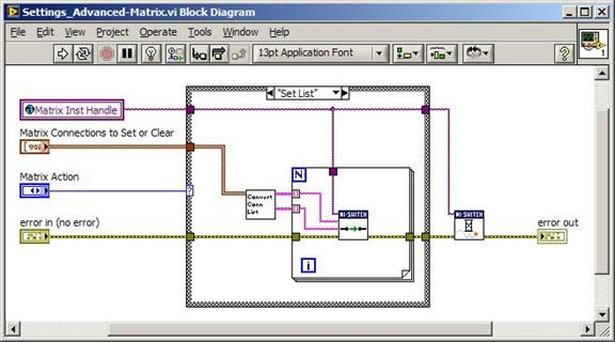 Figure 6. “Set List” mode of Settings_Advanced-Matrix.vi 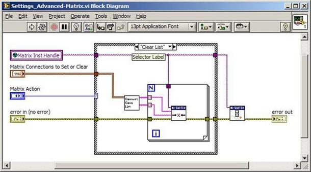 Figure 7. “Clear List” mode of Settings_Advanced-Matrix.vi 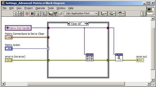 Figure 8. “Clear All” mode of Settings_Advanced-Matrix.vi In Figure 5 you can see the “Matrix Action” enumerated type control that allows the selection of “Set List”, “Clear List” or “Clear All.” It also shows that the VI has the ability to set multiple input to output connections at once and that the inputs and outputs have been assigned meaningful names. Figure 9 and 10 show the strict type defs used for the input and output names. Figure 6 and 7 show the use of a subVI called Convert_Connection_List-Matrix.vi. This VI is shown in Figure 11. 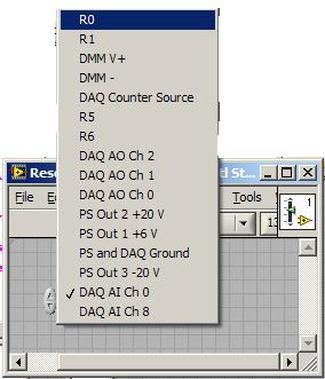 Figure 9. Resource (inputs) control strict type def  Figure 10. Channel (outputs) control strict type def 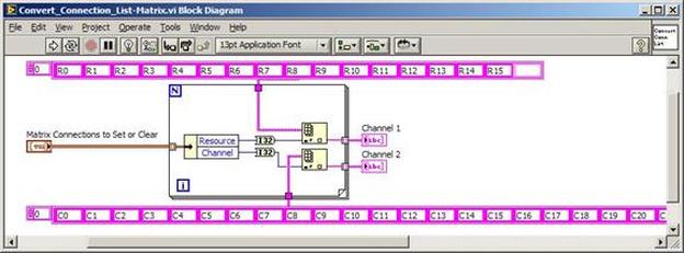 Figure 11. Convert Connection List block diagram Figure 11 shows how the array of meaningful resource and channel names are processed and replaced with the R0… C0… names that the NI driver uses. An additional enhancement that might be considered is if a certain combination of connections could cause damage to the instruments, error checking to prevent those combinations could be added. DMM Now that there is some code in place for making matrix connections we start using some of the other instruments present in the system. The DMM in the system is an NI PXI-4071. For the case of the DMM the drivers supplied from NI are pretty good, they could be wrapped but for my purposes here they will do. Figure 12 shows the block diagram of how to measure the 1k ohm resistor that is at outputs 1 and 2 of the Matrix. 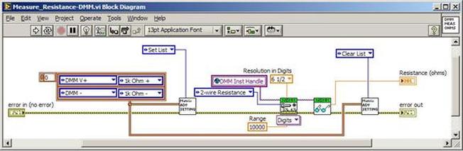 Figure 12. Measure resistance with a DMM through the Matrix. We can see in Figure 12 that the VI, Settings_Advanced-Matrix.vi developed in the last section is used to connect the DMM to the 1k ohm resistor through the matrix. The resistance is measured using the NI drivers niDMM Configure and niDMM Read. Finally, the matrix settings are cleared upon exiting the VI. A good way to ensure you have cleared the same relays you set is to wire the same constant to the set and clear matrix drivers. Figure 13 shows the front panel of the resistance measurement, showing that the VI read 1k ohms (note this is a 5% resistor and that is why it’s off from 1k) 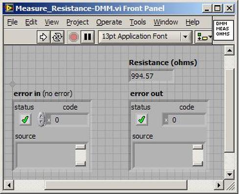 Figure 13. Measure Resistance Example. Now, let’s work in the power supply and use the DMM to measure voltage and current. Figure 14 shows an example of how to use the power supply to force current through the 1k ohm resistor and measure the resulting voltage across the resistor. 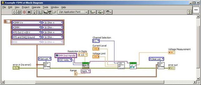 Figure 14. FIMV using the power supply and DMM. Following the code in Figure 14 we see that the matrix is setup to connect the power supply and the DMM to the 1k ohm resistor. The function, resolution and range of the DMM are configured followed by the power supply being set to source the current. Finally, the voltage measurement is taken with the DMM and the matrix settings are cleared before exiting. Figure 15 shows the front panel of the FIMV example. 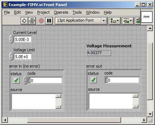 Figure 15. FIMV Example front panel. From Figure 15 we can see that when forcing 5mA through a 1k ohm resistor the result is roughly 5V. Figure 16 shows the code to force voltage and measure current. 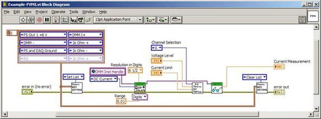 Figure 16 FVMI Example block diagram. In Figure 16 we can see that the matrix settings now apply the power supply to the 1k ohm resistor with the DMM connected in series with the positive power supply lead in order to measure current. The DMM is configured for range, function and resolution, the power supply is configured to force voltage and set the current limit, the current is measured by the DMM and the matrix settings are cleared. Figure 17 shows the front panel of the FVMI example. 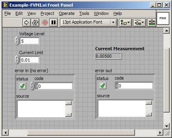 Figure 17. FVMI example front panel. From Figure 17 we see that when 5V is applied to the 1k ohm resistor with a current limit of 10mA, the result is 5mA. Figure 14 and 16 show that I didn’t really develop drivers for the DMM to configure them to measure DC voltage or current, I just use the NI supplied drivers. However, for the application of digitizing a waveform a driver is worthwhile to develop. Two VIs were developed to configure and perform a digitization, Figure 18 shows the block diagram of the digitize configure. 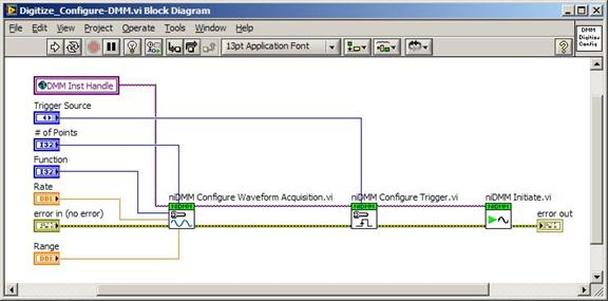 Figure 18. Digitize configure DMM driver. In Figure 18 we can see that there are three NI drivers used. The first is the configure waveform acquisition, this configures the DMM to digitize. Configure trigger, sets the trigger source to various trigger sources like, immediate or external. Finally, the initiate VI tells the DMM to arm and wait for the trigger. Figure 19 shows the front panel of the digitize configure DMM driver. 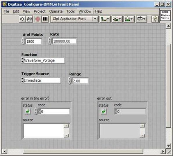 Figure 19. Digitize configure DMM driver. Figure 19 shows all the options that can be set for configuring the DMM to digitize. Most of the options are obvious, the rate is the number of sample per second. The range is the measurement range in the units that match the measurement function. Figure 20 shows the diagram of the digitize VI. 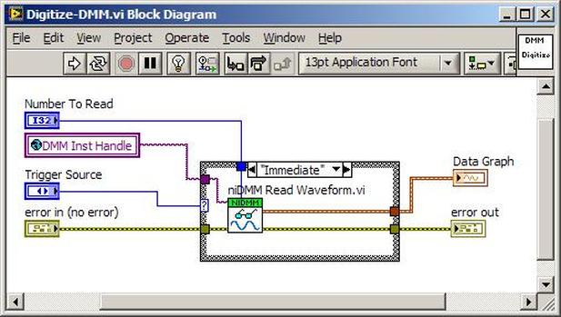 Figure 20. Digitize VI Block Diagram. Figure 20 shows the code that will send the instrument a trigger based on the trigger source and perform the digitization. Figure 21 shows the front panel of the digitize VI with a digitized sine wave being displayed. 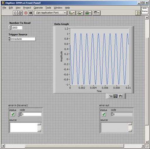 Figure 21. Digitize front panel. Figure 22 and 23 show an example of how to use the digitize drivers with some of the other code that has already been developed to digitize a sine wave. 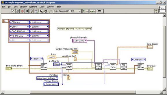 Figure 22. Digitize sine wave example block diagram. 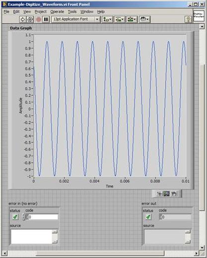 Figure 23. Digitize sine wave example VI front panel. Figure 22 shows the following operations to generate and digitize a sine wave. The first step is to connect the DMM and the DAQ analog output across the 1k ohm resistor. Next, the DMM is configured to digitize for 10ms and the DAQ starts to output a sine wave at 1kHz. Finally, the waveform is digitized, the sine wave output is stopped and the matrix settings are removed. We can see in Figure 23 that since a 1kHz sine wave has a period of 1ms and 10ms were digitized there are ten cycles digitized. Power Supplies While we used the power supply drivers in the FVMI and FIMV code in the DMM section to force the voltage and current we did not look at that code. The system contains the NI PXI-4110 power supply. Figure 24 shows block diagram for the Source DC voltage VI. 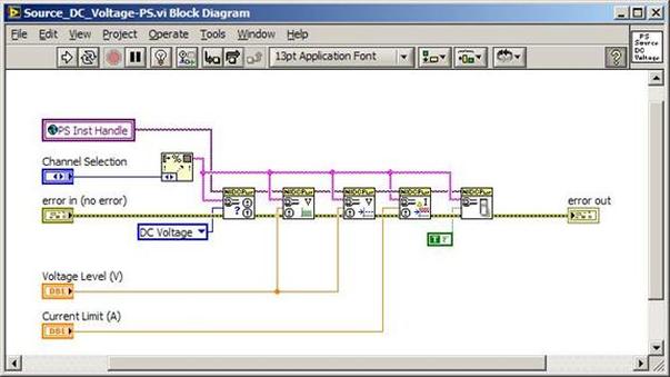 Figure 24 Force DC Voltage block diagram. Figure 24 shows all the NI drivers used to configure and output DC voltage with the power supply. First the power supply function is selected, followed by setting the voltage level and range (the range is automatically set to a predefined level based on the desired voltage level). The current limit is then set and the output enabled. Figure 25 shows the force DC current block diagram. 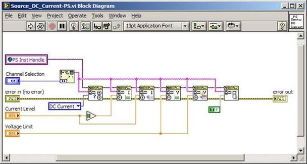 Figure 25. Force DC Current Block Diagram. Figure 25 shows a similar procedure as to set DC voltage. Set the function, set the level and range, set the voltage limit and enable the output. DAQ Again, in the DMM section the DAQ was used to generate a sine wave to digitize but this code was not examined. The system contains a 6259mx m series DAQ. Figure 26 and 27 show the DAQ drivers used to start and stop generating a sine wave. 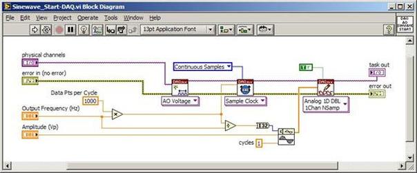 Figure 26. Sinewave Start DAQ VI. Figure 26 shows that it takes three steps to configure a DAQ analog output. First, a physical analog output channel must be selected and configured to output voltage. Next, the sample clock is configured to output data-points at the desired rate. Finally, a sine wave pattern is generated in software and programmed to the DAQ to be output at the previously programmed clock rate. This VI will begin outputting the waveform continuously as the sample clock was programmed to continuous samples. Figure 27 shows the sine wave stop VI. 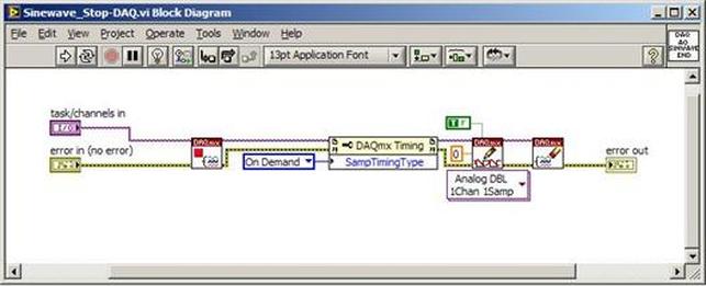 Figure 27. Sinewave Stop VI block diagram. The steps to stop the DAQ output shown in Figure 27 are to stop the task, write a zero to the analog output voltage and clear the task. Figure 28 shows the block diagram of an example of how to use the DAQ to digitize a waveform. 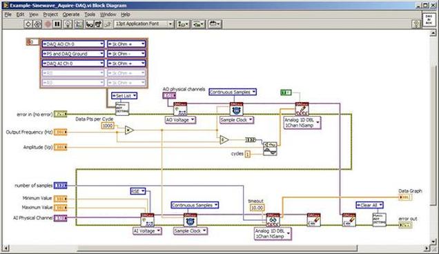 Figure 28. Example of waveform generation and digitization with the DAQ. In Figure 28 we can see that the matrix is used to connect a DAQ analog input to analog output through the 1k ohm resistor. The code to generate the sine wave is the same as from the DMM digitization example. The new code is used to digitize on the analog input and is very similar to the code used to generate the waveform. Replace the analog output channel with an analog input channel. Replace the write channel VI with the read channel VI. Finally, clear both tasks and remove the matrix settings. Figure 29 shows the front panel of the code in Figure 28. 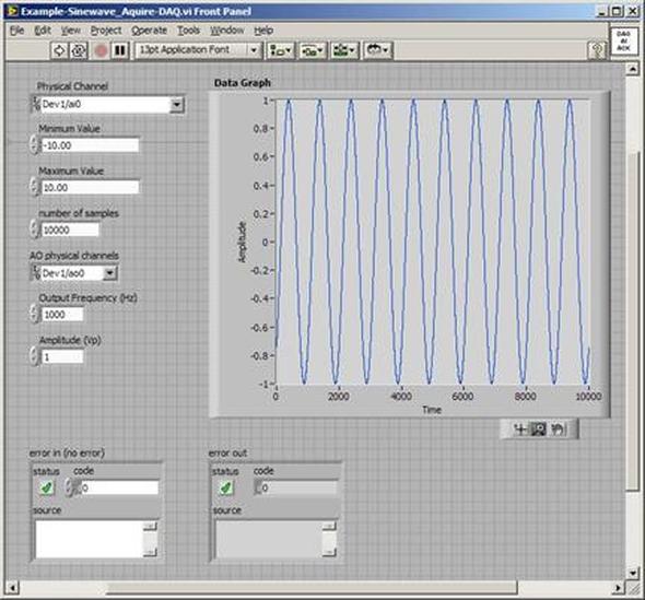 Figure 29. Front panel of digitize waveform with DAQ example
Summary PXI has become the standard for rapid development of flexible, low cost automated test systems. National Instruments with its Labview development environment is the industry heavyweight behind PXI based test. NI provides drivers for their PXI card instruments, however, these drivers can take time to learn and can often require additional work to make them robust instrument drivers. In this entry we saw some examples of how to build these drivers and how to use them to create some useful instrument functions. Some examples included, outputting voltages and currents, connecting instruments via a matrix card, generating waveforms and digitizing waveforms. |
Archives
December 2022
Categories
All

|
 RSS Feed