|
Guard-banding is the concept of tightening test limits by the amount of your measurement accuracy in the measurement system in order to prevent bad DUTs from being mistakenly passed. For example, let’s say you are taking a measurement with a specification limit of 5 volts and the measurement system being used to measure a DUT has a measurement accuracy of 1 volt. To make sure that a DUT with a true value greater than 5 volts does not pass, the limit should be guard-banded by the 1 volt measurement accuracy and set at 4 volts. Here is how this works. You have a DUT with a true value of 5 volts that could be measured anywhere from 4 to 6 volts due to measurement accuracy of 1 volt. See Figure 1. 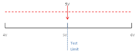
Figure 1. Range of 5V true value with 1 V measurement error.
If the test limit is set at 5 volts according to the specification, then half of the time this DUT will pass and half of the time this DUT will fail. This is an example of a DUT we would want to pass, but might false fail. Now let’s say that there was a DUT with a true value of 5.5 volts. We would never want this DUT to pass but it would pass 25% of the time. See Figure 2. 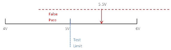
Figure 2. Range of a 5.5V true value with a risk of a false pass.
To avoid the potential of a false pass a guard-band can be applied to create a test limit of 4 volts. Now, with the limit at 4 volts the DUT with a true value of 5.5 volts from Figure 2 can never pass. See Figure 3. 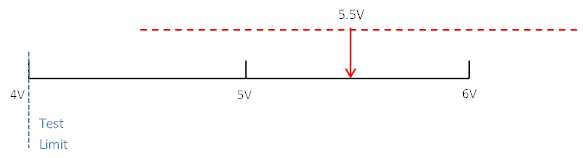
Figure 3. 1 volt guard-band applied to a 5 volt true value.
It’s pretty easy to see that applying a guard-band will potentially fail more good parts. This highlights the importance of knowing where your measurement population is compared to your test limit and having an accurate measurement system. This brings up the concept of CPK which is a measurement to determine if your measurement population is too close to your limit.
0 Comments
Hypothesis testing is an interesting subject. I can’t say that as a test engineer I use hypothesis testing on a regular basis, but it’s a useful thing to know a little bit about. The basic concept is that you have an idea of something being true (a hypothesis) and hypothesis testing coupled with a statistical method to analyze data is used in order to determine if your idea is true. For example, let’s say that under ideal conditions a voltage measurement will always measure 5 volts. Now, I want to know if I make the same measurement in a high humidity environment, will that significantly affect the measurement average. This becomes the null hypothesis and the alternate hypothesis. The null hypothesis is denoted by Ho and in this example is that the voltage measurement in high humidity is equal to 5 volts. The alternate hypothesis is denoted by H1 and is that the measurement under high humidity is not equal to 5 volts. It’s always confusing to me what is supposed to be the null hypothesis. The rule is that the null hypothesis is always assumed to be true. This is confusing because it depends on how you phase the null hypothesis, but here we are interested in a factor (humidity) altering the desired state of measuring 5 volts accurately. It doesn’t really matter what we think is going on. We might think that the humidity does have an effect, but until we can prove it (prove the alternate hypothesis is true) we assume the null hypothesis is true and everything is normal – 5 volts is measured accurately. I kind of think of it as the least interesting or default condition is always the null hypothesis. Example At this point it is easier to just turn the voltage measurement discussion above into an example. I used Labview to generate 100 random numbers to serve as the 5 volt measurements. I intentionally made the data skew slightly above 5 volts. I’m going to use the 1 sample T test in Minitab statistical software to perform the hypothesis testing. I should say that this is kind of trivial example, the real power is when you start using analysis of variance (ANOVA) to look at how multiple factors at multiple levels affect a process. The analysis was performed six times, each time reducing the number of samples that was used. Reducing the samples will illustrate how the decision to reject or fail to reject the null hypothesis becomes less certain. Figure 1 shows a partial screen shot of the data in Minitab. The columns are labeled with the number of samples in that column. 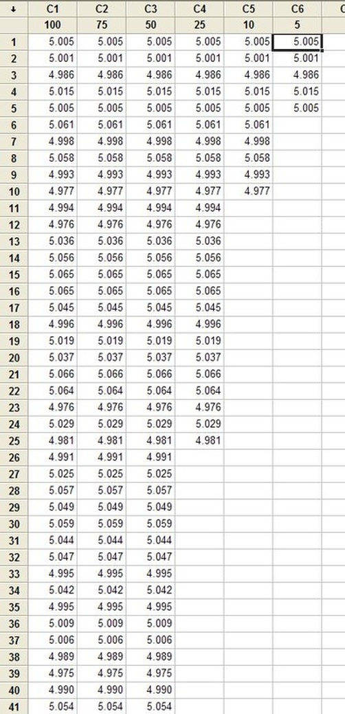 Figure 1. Partial screen shot of measurement data of different sample sizes Figure 2 shows the output of the T test from Minitab. 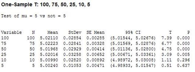 Figure 2. Results for 1 sample T test in Mintab of various sample sizes
In Figure 2 we can see that the column “N” is the number of samples. It shows that mean generally gets closer to 5 with fewer samples. The interesting result here is the P value in the last column. The results are not interpreted by the tool for us, but the rule is that since we are using a 95% confidence interval, any P value less than 0.05 would indicated that we should reject the null hypothesis. So, what’s all that mean? The P value is a probability value that tells us the probability that the null hypothesis is true. For N = 100, 75 and 50 it is saying that there is basically no possibility that the null hypothesis is true and we should reject the null hypothesis in favor of the alternate (and thus the humidity is having an effect). When N = 25 the P value is 0.005, which is still smaller than 0.05 and so we should still reject Ho. For N = 10 and 5 the sample size has gotten small enough that it’s now getting more likely that the mean is in fact 5 V, and we should fail to reject the null hypothesis. Figure 2 shows that we are using a default 95% confidence interval, that’s where the P value cut-off of 0.05 comes from (1 – 0.95 = 0.05). For N = 100, 75, 50 and 25 we are better than 95% confident that the mean is not 5V. You may be wondering why we would do all this. Why not just take a bunch of measurements and calculate the mean? That’s obviously important, but we can always argue that if we take way more measurements (samples) on top the current amount, then the mean will change. That’s why we use this tool, based on the number of samples, we can establish to with some level of confidence weather or not the mean is what we think it is. The results show that we get more and more confident as to the result as we add more samples. Hypothesis testing is also used by manufacturing and quality engineers where you have to sample a value from a process or a production line to try to figure out if the process is at the nominal value or drifting. Summary Hypothesis testing is a useful statistical concept for a test engineer to know and used by a lot of other technical people as well. This was a pretty simple explanation, but hopefully helpful. The steps in hypothesis testing are. 1. Determine your null hypothesis 2. Gather data 3. Assume the null hypothesis is true 4. Determine how much different you sampled values are different from your null hypothesis 5. Evaluate the P value P < 0.05 reject and P > 0.05 fail to reject. The mnemonic device is “If P is low, Ho must go” A statistical concept that comes up often for me as a test engineer is the process capability index. This is a statistical concept that comes from statistical process control and is used on a process that is in control. I don’t really do anything with process control or control charts, but the process capability index is still a useful tool when you are developing tests and need to quickly evaluating a measurement and the feasibility of test limits being applied to it. Cpk When applying test limits to a measurement a design engineer (or someone with more knowledge of the circuit in question) may have an idea of what those limits should be, or they may just be offering a suggestion, making an approximate estimate. In this case, it may be wise to establish a temporary limit to be evaluated when more measurement data is available. Once a good sampling of the measurement data is available the limits can be evaluated to determine if they are going to be capable or if the measurement population is going to be coming very close to the specification limit when the measurement is taken a higher volume in production. Using the process capability index gives a hard number to tell you if you are right up against the specification limit and are going to risk a big fall out if the process shifts. One such process capability index is the Cpk statistic. Here is the formula for Cpk. 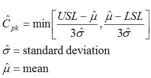 The little hats just mean that these are estimates. Figure 1 shows a plot of 20 measurements of a 5 V power supply (I just made these numbers up for illustration) 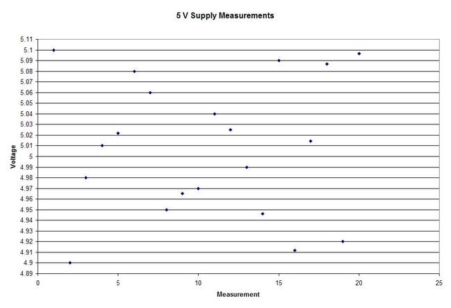 Figure 1. Measurement of a 5 V power supply repeated 20 times. Let’s say that we are measuring a 5 V power supply with an upper and lower specification limit (USL, LSL) set at 1%, 5.05 and 4.95 V. Figure 2 shows these limits marked on the plot. There is obviously some problem here as there are several failures. Calculating Cpk is not really necessary in this case but the result would be:  This is a bad result, any Cpk less than 1 is not good and ideally you want it to be over 2. 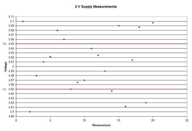 Figure 2. Measurement of 5 V power supply with 1% specification limits. Let’s try 10% limits of 4.5 and 5.5 V as shown in Figure 3. Now we get:  Cpk of 2.545 indicates that the limits are very good and the measurement population is not going to be close to either the low or high limit and is not close to having a lot of failures should the population shift. 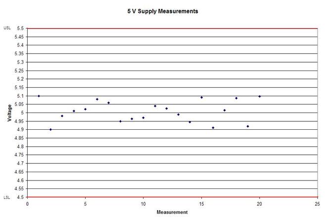 Figure 3. Measurement of 5 V power supply with 10% specification limits.
Now obviously Cpk is not the only factor in setting limits. You don’t just expand the limits if the Cpk is less than 2. The limits would ideally be calculated based on the component tolerances and using a monte carlo type analysis. However, the Cpk is useful in evaluating if a measurement is accurate and if it can be expected to have failures when under higher volume manufacturing. Summary The process capability index is a statistical concept taken from process control that is useful for test engineers to evaluate limits and measurement performance. Cpk is one method of calculating the process capability index. Cpk will help to evaluate how close a measurement population is to either the lower or upper limit. This is useful in predicting future test failures and determining if the measurement accuracy can or should be improved. If we start talking about reliability instead of test engineering we are entering a whole different field of engineering. A test engineer is typically tasked with making sure a product is good when it goes out the door, the reliability engineer is concerned with trying to predict if a product will have a full useful life period. All electronics eventually fail if they are put to use. It may take a few minutes or decades. Since the job of a test engineer is to weed out the failures and defects it’s worthwhile for every test engineer to know a little bit about how products fail. The Bathtub Curve Reliability engineering involves heavy use of statistics and statistical distributions. One of the most fundamental distributions of how products fail is the “bathtub curve.” The idea of the bathtub curve, shown in Figure 1, is that a product goes through three general periods of failure rate. The three periods are, early life or infant mortality, the useful life period and the wear-out period. 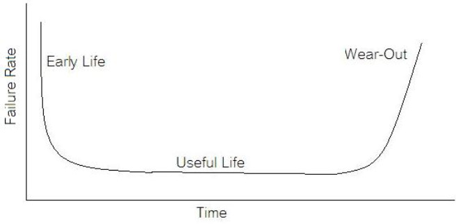 Figure 1. The Bathtub Curve Figure 1 is pretty intuitive, in the early life period the failure rate is decreasing. This behavior is a result of weak products built with manufacturing defects that fail early. When all of those products have failed the failure rate is a constant low value for a long time until the product starts to wear out and the failure rate goes up again. Keep in mind that the curve is the average of a large population of the same product. The early life failure rate still might be very low, but it’s relatively higher than the useful life rate. There is a lot more theory and thought behind the bathtub curve than I’m going to try to go over, because I’m not really concerned with that. There is also some controversy about whether the bathtub curve is realistic or not. The thinking seems to be that the curve could not start out with a decreasing failure rate in the early life period. Even if the early life failures occur very quickly, they did work for a short time and the failure rate should be going quickly up before decreasing (Figure 2). I can see this point, but I think regardless of the most accurate model, the concept of higher, lower, higher failure rates is valid. What I am concerned with is if we accept the idea that there are higher initial failure rates, what can test engineering do about it. 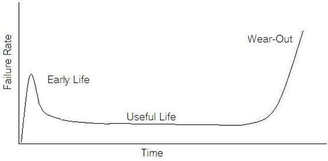 Figure 2. Modified Bathtub Curve: Increasing initial failure rate. Accelerated Life Testing
Accelerated life testing or burn-in are general terms for testing that is designed to stress a product and reveal the early life failures before they can make it to the field. Some techniques include: high temperature operation, temperature cycling, humidity cycling, power cycling, elevated voltage level testing and vibration testing. Burn-In Burn-in, again, is a somewhat broad term. It might mean that a product will operate under normal conditions for some period of time or that it is operated under some set of severe conditions. The idea of operating the product under severe conditions, like high temperature, is to accelerate the process of finding early life failures. It may be the case that performing burn-in tests weakens good products as well as finding the faulty ones. This doesn’t mean that the whole thing is a waste, it can be helpful in determining the general failure rate of the product and the burn-in failures can be analyzed to determine what the underline defect was. It is difficult to determine if it is worth-wile to setup a burn-in test step(s) when a product is manufactured. A big decision when using burn-in techniques is often when to stop. There has to be a trade off between finding the early life failure and just using up the useful life of good products. The cost of setting up a burn-in system should also be considered. Do you want to spend a lot of money and take a lot of time when burn-in just seems like a good idea? There is also a value lost in useful life and time that a product spends in burn-in during manufacturing. To use burn-in you have to have some confidence that the product you are testing will have a higher early life failure rate settling to a low constant later. If the failure rate is just constant or worse always increasing with use of the product, then burn-in is just using up the life of the product and not doing any good to find the weak products. Another criterion for burn-in is the useful life expectancy of the product. Semiconductors can last for decades, but over that time frame they will most likely be obsolete before they wear-out. In this case using up the useful life is not a big problem. Personally, I’m somewhat skeptical of some types of burn-in tests. I think that burn-in is often done simply to give the feeling that everything possible has been done to find failures. If you are working in an industry where the products are hard to replace or man-critical then I can’t really argue too much. But if an occasional field failure is acceptable from time to time, burn-in should be considered more carefully. I also have much more confidence in a burn-in test that performs some type of cycling where materials will be stressed by the changing environment. I’m skeptical of a test where a product is simply operated in constant conditions for some random period of time. Extended Warranty This isn’t exactly a test engineering matter, but knowing a little bit about how products fail gives us some insight into how warranties are used with consumer electronics. The manufacturers warranty usually covers the first 90 days or 1 year, which makes sense and is good, as this should cover the early life failures. However, retailers often want to sell you an extended warranty. Well, the bathtub curve would indicate that this is probably not going to pay off. I also have another way to think about it using a statistical concept called the expected value. Informally, the expected value is what you can expect to happen given two events and two probabilities of those events occurring. Here is the equation: E(x) = x1p1 + x2p2 Where x1 and x2 are some events and p1 and p2 are the probabilities of those events occurring. It’s often stated in the form of a game, like if we bet $5.00 with a 50% probability of winning $5.00 and a 50% probability of losing $5, then what is the average dollar amount we can expect to get? It would look like this: -$5.00(0.5) + $5.00(0.5) = $0 The expected value is $0. Now, if we did this bet only one time we would either win or lose $5.00. However, the idea is to understand of the expected amount we would win or lose if it were possible to make this gamble a very large number of times. It’s pretty simple to see how to evaluate a warranty using the expected value. Let’s say you are going to buy a TV for $500 and the retailer wants to sell you an extended warranty for $100. We don’t know what the probability that the TV will fail will be, but it’s going to be pretty small. Keeping in mind that the larger portion of the failures (early life) will be covered by the manufacturer’s warranty, and then estimate it will fail 1% of the time. The $500 dollars paid for the TV is gone either way. The game to evaluate with the expected value is paying $100 with a chance to “win” $400 (the cost of a $500 replacement TV minus the $100 warranty cost). The expected value looks like this: -$100(0.99) + $400(0.01) = -$95 Pretty good deal for the retailer. For the warranty to start paying off, the percentage of failing TVs has to go up to greater than 20%. It would be remarkably poor quality for a modern piece of consumer electronics to fail 20% of the time after the manufacturers warranty had expired. Declining the warranty, you have automatically accepted the gamble that if the TV fails you will have to replace it at full cost. That would look like this (at 1% failure rate): $0(0.99) + -$500(0.01) = -$5 Either gamble has a negative expected value, but relative to each other -$5 is a much better gamble than -$95. Summary The bathtub may not be a perfect model, but is a useful concept for a test engineer to be familiar with. Accelerated life testing and burn-in, when carefully considered, are an important test strategy tool for test engineering and insuring product reliability. Having a good understanding of statistics is important for a test engineer. There is a lot that can be learned about your tests by examining the results. Some of the important tools are taken from the Six Sigma quality world, but there is so much going on there I could never cover it all. Also, many of the Six Sigma techniques are more focused on manufacturing and preventing waste (lean manufacturing) and achieving high yields. While these issues are of concern to a test engineer, you have to balance the desire for yield with the concern for quality. One statistical topic of particular importance is Gage Repeatability and Reproducibility studies. Also going by the name of Measurement System Analysis, performing a gage study is necessary to determine if and where any sources of variation in a test system are coming from. Sources of Variation There are three main sources of variation Operators When reading about gage R&R operators tend to be discussed as the actual people who are performing the measurements, but they can also be thought of as combination of equipment. If you wanted to look for variation problems with test fixtures or test systems, operators could be thought of as follows: Operator 1 = Test System 1 + Fixture 1 Operator 2 = Test System 1 + Fixture 2 Operator 3 = Test System 2 + Fixture 1 Operator 4 = Test System 2 + Fixture 2 When operators are people, comparing them allows you to identify poor training or a setup that is difficult to reproduce. Measurement System/Method What is being considered here, is the instrument taking a measurement or the test/measurement method. The word “gage,” is like a gage on a meter that shows a measurement, it’s just a substitute for instrument. Parts Ideally, parts should be the main source of variation reveled by the Gage study. When designing a gage study, ideally, all of the parts chosen should represent the entire population of parts by spanning the full range of tolerances. This is not always possible as the availability of parts may be limited or extremes in tolerance may not be available. This is important to see how the system performs on all of the parts that may have to measure. If an instrument or test system can accurately measure at the low range of the parts tolerance, but not towards the upper range that is a linearity problem. Operator by Part There is actually a fourth source, but it’s a combination of the others. Once operator and part variability have been considered, operators can be evaluated on a per part basis. This may reveal that on a particular part all of the operators are unable to measure it consistently. While this would also show up on the part variation, it is more difficult to tell in that case if the variation is a gage repeatability problem or an operator problem (due to that part). Other than part-to-part all of the sources of variation can be classified as problems due to repeatability or reproducibility. Repeatability Repeatability is defined as variation due to instrument error. Of the sources of variation listed above Measurement System/Method is assessed by examining the repeatability. What is done is a part is measured several times without changing any of the setup or operators. That data is then used to quantify the variation in a measurement system resulting from an instrument or test method. Reproducibility Reproducibility is defined as the variation due to external sources such as operators and environmental conditions. Of the sources of variation listed above Operators and Operators by Part are assessed by examining the reproducibility. Here, several operators will measure the same part repeatedly. This will reveal variability due to the operators. Example R&R Studies In order to show some of the features and problems that can be found, I’ll do an example of a simple R&R study and alter the data to show some features. Setup I’m going to measure ten 1k ohm resistors five times each, with two operators, and analyze the results with Minitab statistical software. In an ideal gage the parts should represent the complete population of parts, so if I use 1k 5% resistors I should have some in my experiment that measure at the tolerance extremes (950 ohm to 1050 ohm). Experiment 1: Measured Data The first experiment was to gather the data and analyze the results. I used two Fluke 189 DMMs to measure the resistance and act as the two operators. Figure 1 shows the data. 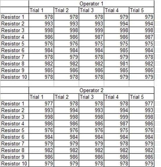 Figure 1. Original measured resistance data Figure 1 shows that I could not find a representative resistor population of the tolerance. As stated, the tolerance is 5% giving a range of resistances of 950 to 1050. However, none of the resistors in this population were even at 1k. This isn’t ideal but I wanted to use real data for the first experiment. Figure 2 shows the Minitab result of the crossed ANOVA gage study. 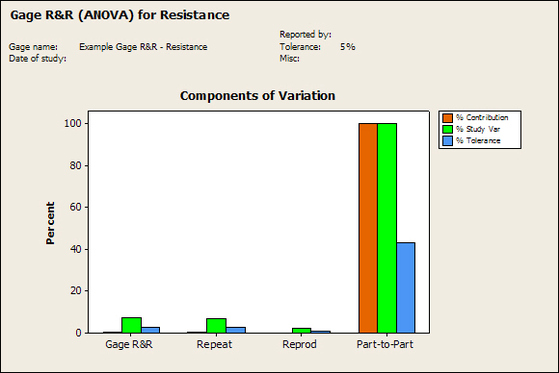 Figure 2. Gage R&R results. Figure 2 shows that the vast majority of the variation found was due to part to part variation. This is what we want to see when evaluating our test system. Figure 3 is another plot from this same experiment. It also shows the variation due to the parts with a connected box plot. 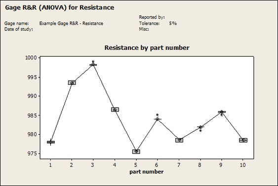 Figure 3. Connected box plot by part number. Figure 3 shows a connected box plot where a box plot shows the following. Outliers are shown as a star (*). The upper whisker extends to the maximum data point within 1.5 box heights from the top of the box. The box itself shows, the median, the first and third quartile. The first quartile shows where 25% of the data is less than or equal to the bottom line. The median is where 50% of the data are less than or equal to the center line. The third quartile is where 75% of the data are less than or equal to the top line. The lower whisker extends to 1.5 box heights below the bottom of the box. The connection line shows the averages. Figure 4 shows the connected box plot by operator. 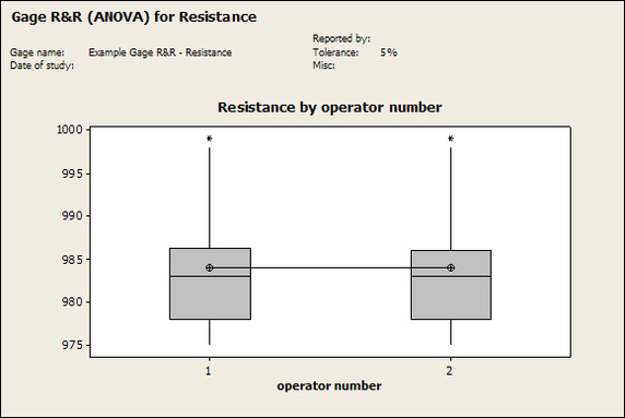 Figure 4. Connected box plot by operator number. In Figure 4 it you can see that it is showing an outlier on the high side. This is really illustrating the poor population I have for a 1k resistor since it is flagging a value below 1k as an outlier. We can also see that the reproducibility was very good from this plot, as both operators look about identical. Experiment 2: Problem with part 1 For this experiment I have altered the data for part 1 to make it look like it had some sort of repeatability issue. Figure 5 shows the new part 1 data. 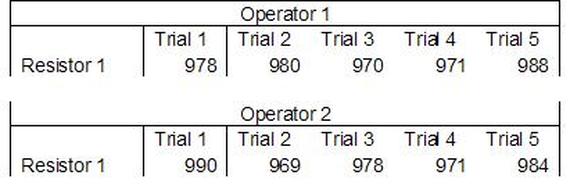 Figure 5. Altered part 1 data. Figure 6 shows the ANOVA gage study result with altered part 1 data. 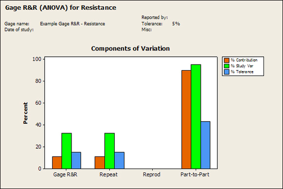 Figure 6. ANOVA gage study with altered part 1 data Figure 6 shows that there is now a more significant portion of variation due to repeatability, but we have to look at some of the other plots to understand what is really happening. Figure 7. shows the connected box plot by part number. 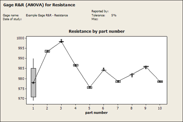 Figure 7. connected box plot by part number with altered part number 1 data So, now we can see from Figure 7 that there was something wrong with the repeatability of part 1. With this new data we can conclude that there is probably something going on with part 1 since it cannot be measured accurately repeatedly. We should also check that this problem was not due to just one of the operators and Figure 7 wouldn’t necessarily show this. Figure 8 shows the Xbar and R Chart for the experiment. 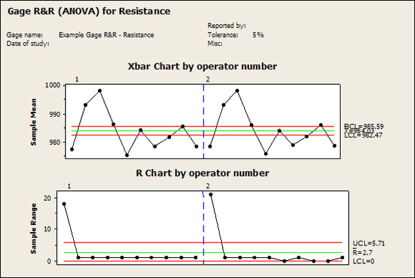 Figure 8 Xbar and R Chart with altered part number 1 data. Figure 8 shows us that both of the operators measured a large range of values (R Chart). This tells us that both of the operators had trouble measuring this part accurately. The Xbar chart shows the averages of all the parts by operator along with the grand average and upper and lower control limit line. The R (Range) chart shows the range of measurements made and plots them with the average range and control limits. We can see in Figure 8 that the range for part 1 on operator 2 was up over 20 ohms. Experiment 3: Repeatability Problems For this experiment I have altered all of the original data so that each measurement was offset by either plus or minus five ohms. Figure 9 shows the data set used. 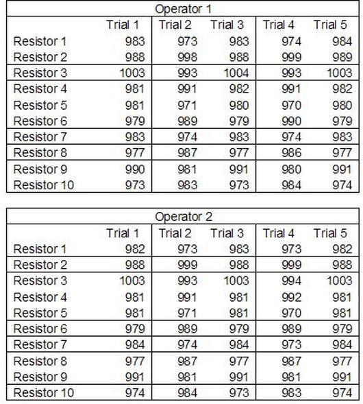 Figure 9. Resistance measurement data with added offset Figure 10 shows the ANOVA gage study result with offset data. 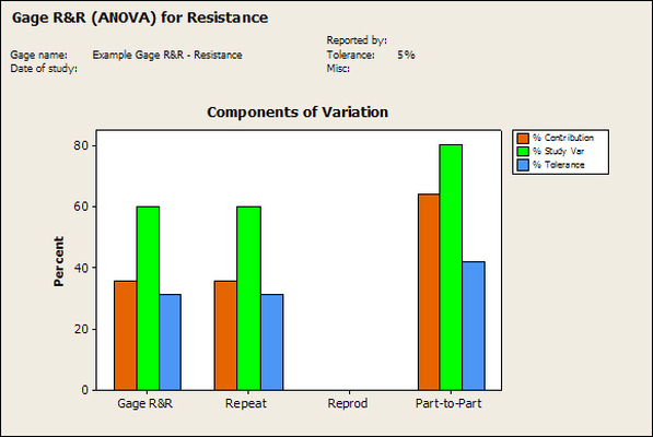 Figure 10. shows the ANOVA gage study result with offset added From Figure 10 it can be seen that the repeatability is a significant source of variation and may be a problem that needs investigating. This test system may not be making very accurate measurements. Figure 11 shows the resistance by part number. 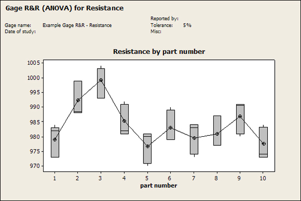 Figure 11 Resistance by part number for data with offset added. Figure 11 shows the large boxes in the box plot indicating a larger spread in the resistance measurements that is consistent for each part, indicating a repeatability problem. Experiment 4: Reproducibility Problem For this experiment the original data was again modified, this time an offset of plus eight ohms was added to all of the operator 2 data. Figure 12 shows the new data set. 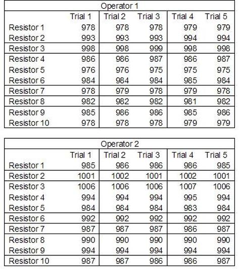 Figure 12. Resistance measurement data with +8 ohms on added to operator 2 Figure 13 shows the ANOVA gage study results. 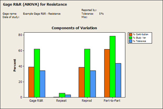 Figure 13. ANOVA gage study results with +8 ohms added to operator 2 From Figure 13 we can see that the reproducibility is now a significant portion of the variance and repeatability is back down. Figure 14 shows the resistance by operator number. 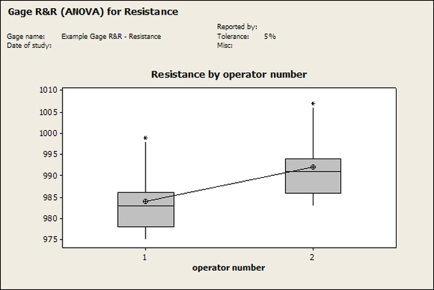 Figure 14. Resistance by operator number with +8 ohm offset added to operator 2 Figure 14 shows the 8 ohm shift nicely and would help to identify a reproducibility problem. Figure 15 shows the operator by part interaction. 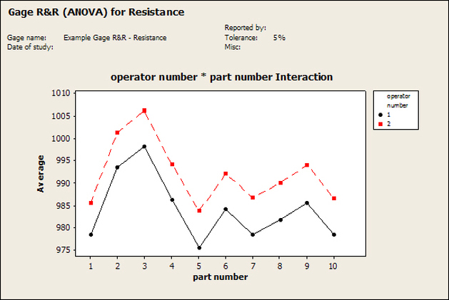 Figure 15. Operator by part interaction with +8 ohm offset added to operator 2
Figure 15 also shows that operator 2 consistently measures the resistances higher than operator 1, again showing reproducibility problems. Other Thoughts Using Minitab is nice for performing these studies because you get lots of plots in just a few clicks, but it is pretty formal and isn’t really necessary to learn about your test system. Just designing the study, taking the data and doing some quick plots in Excel is usually all you need to figure out what needs more investigation. Minitab also gives you a lot of quantitative data, like a p-value for each of the sources of variation. The idea with the p-value is you hypothesize that, for example, repeatability is not a significant source of variation and then the resulting p-value (low p = reject the hypothesis) tells you if that hypothesis is correct. This is probably more useful if you have to present your results in a formal way. Summary Performing a gage study can reveal a lot about your test system you will need to know before you can feel comfortable with the test results it is producing. The sources of variation are part-to-part, measurement system/method (repeatability) and operators (reproducibility). Often times you have to look at the same data presented in many different ways to see the patterns and get the full picture of the problems. While, gage studies reveal problems, that is just the start, it’s still up to you to go figure out what is causing the problem and how to correct it. |
Archives
December 2022
Categories
All

|
 RSS Feed